How to Use Excel VLOOKUP Function in Office 365?

Excel VLOOKUP Function:

In this tutorial, we demystify the description, basic syntax, and usage of the Excel VLOOKUP function in Office 365. Get an official version of Microsoft Excel from the following link: https://www.microsoft.com/en-in/microsoft-365/excel.

Description of the VLOOKUP Function:

• The VLOOKUP (Vertical Lookup) function is used to look up data in a range or table by row.
• It searches for a value in the first column of a table and returns the value in the same row as per the col_index_num position.
• This function supports exact match, approximate match, and wildcards (*?) for partial matches.

VLOOKUP Function – Syntax:

The basic syntax of the VLOOKUP function is,

=VLOOKUP(lookup\_value, table\_array, col\_index\_num, [range\_lookup])

Argument Explanation:

• 1) lookup_value (Required) – The value that you want to search for must be in the first column of the given range that you specify in the table_array argument.
• 2) table_array (Required) – It is the range of cells that needs to be two or more columns of data. The range should contain the lookup_value and return value.
• 3) col_index_num (Required) – It is the column number in the given range that contains the return value. The counting starts from the leftmost column (i.e. first column is 1) in the table array.
• 4) range_lookup (Optional) – A logical value either TRUE or FALSE.
  • TRUE (1) – Approximate match: It looks for the closest value in the first column with the look_up value by assuming the first column in the table is sorted either alphabetically or numerically. It is the default match if you don’t specify this argument.
  • FALSE (0) – Exact match: – It looks for the exact match in the first column with the look_up value.
• Refer to the below screenshots to understand the arguments in pictorial representation.

First Argument:

Second Argument:

Third Argument:

Fourth Argument:

Diverse Purposes of VLOOKUP:

| Looks only Right | Column Numbers | Case-insensitive | Exact Match |
| Approximate Match | First Match | Wildcard Match | Two-way Lookup |
| Lookup a Value

from Another Sheet **| Lookup a Value

from Another Workbook | INDEX and MATCH** |

1) VLOOKUP – Looks only Right:

• VLOOKUP function can only lookup right.
• The value that you want to look up must be in the first column of the given cell range.
• The result values that you want to retrieve can appear in any column to the right of the lookup values.

Example 1:

• In this example, we have looked up a value ‘Robert’ in the “First Name” column.
• Here, the column index argument is 2 , so as per the cell reference, the VLOOKUP function looks right from the leftmost column (First Name), and returned the output as ‘John’ from the 2nd column (Last Name).

Example 2:

• In this example, we have looked up a value ‘Betty’ in the “Last Name” column.
• Here, the column index argument is 3 , so as per the cell reference, the VLOOKUP function looks right from the leftmost column (Last Name), and returned the output as ‘Texas’ from the 3rd column (State).

2) VLOOKUP – Column Numbers:

• When you are using the VLOOKUP function, assume that every column in the table is numbered starting from the left towards right.
• If you want to get an output from a specific column , you have to provide the relevant number as the column index argument.
• For example, if you want to retrieve output from the column that is second from the lookup column, then you have to give the column index argument as 2.

Example 1:

• Here, in this example, we have looked up a value ‘1105’ in the “ID” column and retrieved the value from the “Last Name” column that is 3rd from the “ID” column.
• As the “Last Name” column is 3rd from the lookup column, we have given the column index as 3.
• The function returned the output as ‘Linda’ corresponding to the lookup value ‘1105’.

Example 2:

• Here, in this example, we have looked up a value ‘Kenneth’ in the “Last Name” column and retrieved the value from the “Salary” column that is 2nd from the “Last Name” column.
• As the “Salary” column is 2nd from the lookup column, we have given the column index as 2.
• The function returned the output as ‘34808’ corresponding to the lookup value ‘Kenneth’.

3) VLOOKUP – Case-insensitive:

• The VLOOKUP function performs a case-insensitive lookup within a table or cell range.

Example:

• We are going to look up a value ‘SUSAN’ in the “First Name” column.
• If the lookup value is present inside the table, we are going to retrieving the value from the “Last Name” column that is 2nd from the “First Name” column as a result.

• As the VLOOKUP function is case-insensitive, it looks up for susan, SUSAN, Susan, sUsan, etc in the “First Name” column.
• The function returned the output as ‘Ava’ as it locates the Susan (first occurrence) in the third row and so the value SUSAN is ignored.

VLOOKUP TRUE vs FALSE:

4) Exact Match (FALSE):

• The VLOOKUP function looks up for the exact match in the first column (leftmost column) of the table or cell range if the range_lookup argument is given as FALSE.
• You can also give zero (0) instead of FALSE.
• If the function can’t able to find the exact match in the first column, it returns a #N/A error.

Example:

• The function looks for an exact match with the lookup value ‘1108’ in the given cell range as the argument is declared as FALSE.

• If the value 1108 is present within the cell range, then the function returns the value in the 4th column corresponding to the same row of the lookup_value.

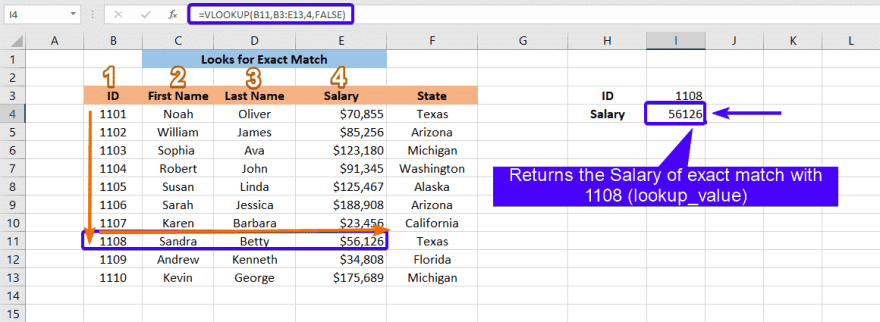
• So, for this example, it returned the output as ‘56126’.

5) Approximate Match (TRUE):

• Sometimes, you may not require the exact match , and in that case, you can use the *TRUE argument * so the function looks up the closest match.
• If you set the argument as TRUE or omitted , it will search for an exact match first and if an exact match is not found, it looks for the next highest value that is less than the lookup value.
• You can also give one (1) instead of TRUE.
• By default , it will take the argument as TRUE if you omit the argument.
• If the lookup value is smaller than the smallest value in the lookup range, the Excel VLOOKUP function will return the #N/A error.

Example:

• In this example, the VLOOKUP function looks up for the value 1120 in the first column (leftmost column) of the table.
• Although the value 1120 is not present at the table it will not throw any error as we have given the argument as TRUE (approximate match).

• There is no value 1120 in the first column so it tells the function to return an approximate match.

• So, in this example, the value will be 1110 (next highest value less than the lookup value) and it returns the salary output as ‘175689’ (4th column) of the same row.

6) First Match:

• If the lookup column or leftmost column contains identical or duplicate values , then the function considers the first occurrence and returns its corresponding row output.

Example:

• Take a look at the example below. The VLOOKUP function is configured to find the salary for ‘William’.

• There are two entries with the first name William so the function returns the salary of the first entry, 85256 , and ignored the second instance.

7) Wildcard Match:

• If you want to perform a partial match with the use of the Excel VLOOKUP function, you have to make use of wildcards.
• In simple words, you can give a part of a value that you want to search for when you don’t remember the exact value.
• To use wildcards, you have to specify the last argument as FALSE for exact match mode.
• To match any sequence of characters , you have to use Asterisk(*).
• Use a Question mark (?) to match any single character.

Using Asterisk (*):

Example 1: Searching for a value that starts with certain characters

• In this example, we have looked up a value that starts with ‘Kev’ in the “First Name” column.

• The function found the value ‘Kevin’ in the First Name column so it returns the state as ‘Michigan’.

Example 2: Searching for a value that ends with certain characters

• In this example, we have looked up a value that ends with ‘es’ in the “Last Name” column.

• The function found the value ‘James’ in the Last Name column so it returns the salary as ‘85256’.

Example 3: Searching for a value that starts and ends with certain characters

• In this example, we have looked up a value that starts with ‘je’ and ends with ‘ca’ in the “Last Name” column.

• The function found the value ‘Jessica’ in the Last Name column so it returns the state as ‘Arizona’.

Example 4: Searching based on cell value

• You can also enter the known part of the value in some cell, say I3, and combine the wildcard character with the cell reference using an ampersand (&).
• In this example, we have looked up a value that starts with ‘Rob’ in the “First Name” column.
• We have entered the known part of the first name value in cell I3 for referring it to the formula.

• The function found the name ‘Robert’ in the First Name column so it returns the salary as ‘91345’.

Using Question Mark (?):

• If you don’t know even what kind of characters present inside the table but you know the number of characters then, you can use the question mark instead of an asterisk to search for a specific number of characters.

Example: To search for a four-character value

• In this example, we have looked up for a four-character value in the “First Name” column.

• In the First Name column, “Noah” is the four-character value so the corresponding row salary ‘70855’ is returned as output.

8) VLOOKUP – Two-way Lookup:

• Generally, in the Excel VLOOKUP function, you have to give a static number for the column index argument.
• But, you can also create a dynamic column index with the use of the MATCH function. This sort of technique assists you to match both rows and columns by creating a dynamic two-way lookup.

Example:

• In this example, VLOOKUP is configured to perform a lookup based on ID and Salary.
• For the column index argument, we have used the MATCH function to get the position of the column “Salary”.

• We have looked up a value ‘1107’ in the “ID” column and retrieved the salary ‘23456’ as output.

9) VLOOKUP – Lookup a Value from Another Sheet:

• It is possible to look up a value from the table that is on another sheet by using the Excel VLOOKUP function.
• To refer a table on another sheet, you have to add the sheet name and an exclamation mark before the table/cell range.

Example:

• Refer to the below screenshot that shows the Sheet9.

• In Sheet10, we have entered the VLOOKUP formula to search for the ‘1106’ ID in Sheet9.

• The ID ‘1106’ is present in the Sheet9 and so the function retrieved the “First Name” of its corresponding row from the Sheet9, ‘Sarah’ , and displays the output in the Sheet10.

11) INDEX and MATCH:

• In order to perform advanced lookups, you can use INDEX and MATCH functions instead of using VLOOKUP.

Example:

• Using the MATCH function, we have searched for an exact match with ID ‘1104’ within the given cell range.

• If the ID is present within the cell range, it will retrieve the State of its corresponding row and for that purpose, we have used the INDEX function.

• It retrieved the state ‘Washington’ as output for the ID ‘1104’.

Common Errors:

• #N/A error – If the range_lookup is FALSE and can’t able to locate the exact match within the cell range, the VLOOKUP function returns this error.
• #REF! error – You will get this error value if the col_index_num is greater than the number of columns.
• #VALUE! error – This error will be returned if the table_array is less than 1.
• #SPILL! error – If the formula depends on the implicit intersection for the lookup value and uses a whole column as a reference, you will acquire this error value.
• #NAME? error – To search for a person’s name, you have to use quotes around the name in the formula, or else you will get this error.
• You may get the wrong result if range_lookup is TRUE or omitted, the first column needs to be sorted numerically or alphabetically. You will not get the expected return value if the first column is not sorted. Use either FALSE for an exact match or sort the first column.

Closure:

Searching for data in a table or cell range is actually easy and simple with the use of the VLOOKUP function. We hope that the above article assisted you to learn all about the Excel VLOOKUP function in Office 365. The description, syntax, and diverse scenarios of VLOOKUP function explained distinctly for your easy understanding.

Drop your valuable queries/feedback in the below comment section. Thanks for visiting Geek Excel!! Keep Learning with us!!

Read Ahead:

• How to Vlookup Values from Bottom to Top in Excel 365?
• “Find Next Match” Shortcut in Microsoft Excel 365 – Quick Shortcuts