Normally, we can look up and return a matching value from a range of data by using the LOOKUP function. In this tutorial, we will talk about how to lookup the entire row and return the value based on certain criteria in Excel by using the INDEX and MATCH functions. Let’s get started!! Get an official version of ** MS Excel** from the following link: https://www.microsoft.com/en-in/microsoft-365/excel
Generic Formula:
- Use the below formula to look up and retrieve an entire row in Excel.
=INDEX(data,MATCH(value,range,0),0)
Syntax Explanations:
- INDEX – The INDEX function returns the value at a given position in a range or array.
- MATCH – In Excel, this function will locate the position of a lookup value in a row, column, or table. Read more on the MATCH function.
- Comma symbol (,) – It is a separator that helps to separate a list of values.
- Parenthesis () – The main purpose of this symbol is to group the elements.
- Range – It represents the input ranges in your worksheet.
- Value – It is the criteria that want to get the values.
- *Data * – It is the input range from your worksheet.
Practical Example:
Now, we are going to see the steps to find the value from the entire row based on the given criteria.
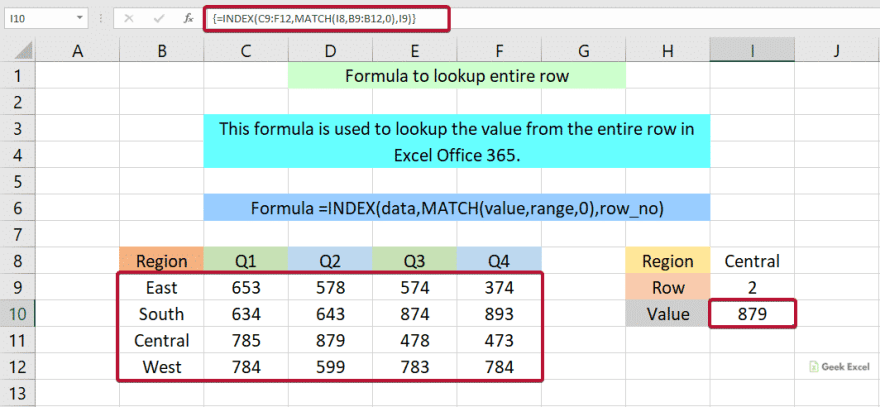
- First, we will give the input values from Column B to Column F.

- Here, we need to find the value based on the given criteria shown below.

- Enter the formula in the formula bar section.

- After that, Press CTRL + SHIFT + ENTER Keys.
- Finally, it will find and return the value based on the given criteria. Refer to the below image.

Wrap-Up:
From this short tutorial, we have described the simple formula used to lookup the entire row in Excel by using the INDEX and MATCH functions. Hope you like it. Please state your query in the below comment section. We will assist you. Click here to know more about Geek Excel!! And Excel Formulas!!


Top comments (0)