DEV Community

Cover image for Neural networks 101: The basics of forward and backward propagation
Daniel Cooper
Daniel Cooper

Posted on • Updated on

Neural networks 101: The basics of forward and backward propagation

This post shows you how to construct the forward propagation and backpropagation algorithms for a simple neural network. It may be helpful to you if you've just started to learn about neural networks and want to check your logic regarding the maths.

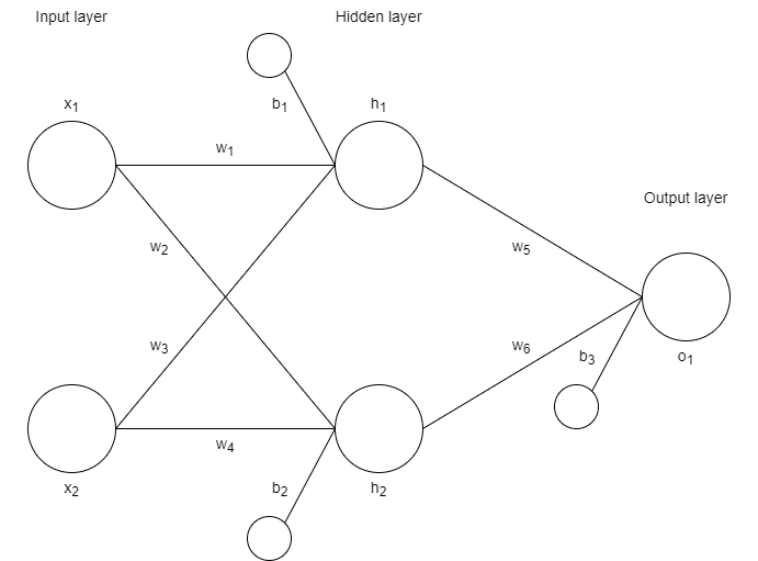
Consider the neural network below. It has two inputs (x1 and x2), two hidden neurons (h1 and h2), one output neuron (o1) and a series of weights and biases.

Our neural network

We want to use this neural network to predict outputs and have four training examples which show the expected output y for different combinations of x1 and x2.

x1 x2 y
0 0 0
0 1 1
1 0 1
1 1 1

Our neural network starts with a random set of weights between 0 and 1, and biases set to 0. In this initial configuration, as you might expect, our neural network will predict outputs which bear no relation to the expected outputs.

To improve the prediction accuracy, we need to optimise the weights and biases so that they work together to predict outputs that are as close as possible to the expected outputs.

This optimisation process is called training and it involves two stages: forward propagation and backpropagation.

Forward propagation

The forward pass stage moves through the neural network from left to right.

Each neuron is configured to sum its weighted inputs with its bias and to then pass that value z through an activation function σ\sigma to produce an output a.

Our neural network with z and a for each neuron

We can express the sum z and output a for each neuron as:

zh1=w1x1+w3x2+b1ah1=σ(zh1)zh2=w2x1+w4x2+b2ah2=σ(zh2)zo1=w5ah1+w6ah2+b3ao1=σ(zo1) \begin{align*} z_{h1} &= w_1x_1 + w_3x_2 + b_1 \newline a_{h1} &= \sigma(z_{h1}) \newline\newline z_{h2} &= w_2x_1 + w_4x_2 + b_2 \newline a_{h2} &= \sigma(z_{h2}) \newline\newline z_{o1} &= w_5a_{h1} + w_6a_{h2} + b_3 \newline a_{o1} &= \sigma(z_{o1}) \end{align*}

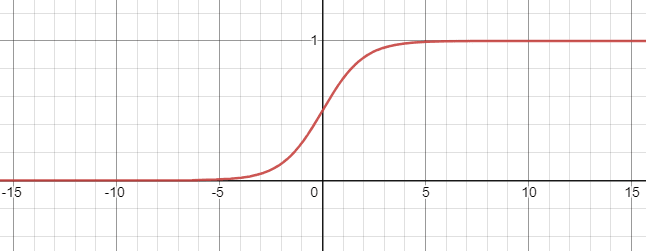
The activation function σ\sigma is used to transform a continuous input into an output between 0 and 1, with 0 for large negative inputs and 1 for large positive inputs.

Here we'll apply the commonly-used Sigmoid function for activation:

σ(z)=11+ez \sigma(z) = \frac{\mathrm{1} }{\mathrm{1} + e^{-z}}

Sigmoid activation function

With these equations, we can use the x1 and x2 from each of the training examples to predict an output (ao1).

To measure the prediction accuracy of our neural network across all of the training examples, we can the Mean Squared Error function to find the total loss J:

Total loss, J=12mi=1m(ao1y)2 \displaystyle \text{Total loss, J} = \frac{1}{2m}\sum_{i=1}^{m}(a_{o1} - y)^2

where m is the total number of training examples; in our case, m = 4.

To begin, the total loss J is almost certain to be greater than zero unless we have been particularly fortunate with our random weights and biases.

More likely we will need to optimise the weights and biases and to do that, we use backpropagation.

Backpropagation

Backpropagation moves backwards through the neural network, from right to left.

Using equation from above for the total loss J, if we consider just a single training example with m = 1, we can define a loss L:

Loss, L=12(ao1y)2 \displaystyle \text{Loss, L} = \frac{1}{2}(a_{o1} - y)^2

The loss L is dependent on ao1 which itself is dependent on all of the weights and biases. It follows that optimising these weights and biases will reduce the loss L.

Using an iterative process, we can optimise each weight and bias using the principle of gradient descent and a suitable learning rate α\alpha :

ws=wsαdLdws where s = 1, 2, ..., 6bt=btαdLdbt where t = 1, 2, 3 \begin{align*} w_s &= w_s - \alpha\dfrac{\mathrm{d}L}{\mathrm{d}w_s} \text{ where s = 1, 2, ..., 6} \newline\newline b_t &= b_t - \alpha\dfrac{\mathrm{d}L}{\mathrm{d}b_t} \text{ where t = 1, 2, 3} \end{align*}

To use these equations, we first need expressions for the derivative of the loss L with respect to each weight and bias. These expressions are partial derivatives which we can derive using the chain rule.

Before we start, there are two derivatives that we will come in handy. The first is the derivative of the Sigmoid activation function:

σ(z)=11+ezdσ(z)dz=σ(z)(1σ(z)) \begin{align*} \sigma(z) &= \frac{\mathrm{1} }{\mathrm{1} + e^{-z}} \newline\newline \dfrac{\mathrm{d}\sigma(z)}{\mathrm{d}z} &= \sigma(z)(1-\sigma(z)) \end{align*}

The second is the derivative of the loss L with respect to ao1:

L=12(ao1y)2dLdao1=(ao1y) \begin{align*} \displaystyle L &= \frac{1}{2}(a_{o1} - y)^2 \newline\newline \dfrac{\mathrm{d}L}{\mathrm{d}a_{o1}} &= (a_{o1} - y) \end{align*}

Let's now start with weight w6 and find the derivative of loss L with respect to w6:

dLdw6 \dfrac{\mathrm{d}L}{\mathrm{d}w_6}

Using the chain rule, we can say that:

dLdw6=dLdao1.dao1dw6 \dfrac{\mathrm{d}L}{\mathrm{d}w_6} = \dfrac{\mathrm{d}L}{\mathrm{d}a_{o1}}.\dfrac{\mathrm{d}a_{o1}}{\mathrm{d}w_6}

Therefore:

dLdw6=(ao1y).dao1dw6 \dfrac{\mathrm{d}L}{\mathrm{d}w_6} = (a_{o1} - y).\dfrac{\mathrm{d}a_{o1}}{\mathrm{d}w_6}

This is progress but we need to go further with:

dao1dw6 \dfrac{\mathrm{d}a_{o1}}{\mathrm{d}w_6}

Using the chain rule again, we can say:

dao1dw6=dao1dzo1.dzo1dw6 \dfrac{\mathrm{d}a_{o1}}{\mathrm{d}w_6} = \dfrac{\mathrm{d}a_{o1}}{\mathrm{d}z_{o1}}.\dfrac{\mathrm{d}z_{o1}}{\mathrm{d}w_6}

where:

dao1dzo1=dσ(zo1)dzo1=σ(zo1)(1σ(zo1)) \dfrac{\mathrm{d}a_{o1}}{\mathrm{d}z_{o1}} = \dfrac{\mathrm{d}\sigma(z_{o1})}{\mathrm{d}z_{o1}} = \sigma(z_{o1})(1-\sigma(z_{o1}))

and:

dzo1dw6=d(w5ah1+w6ah2+b3)dw6=ah2=σ(zh2) \dfrac{\mathrm{d}z_{o1}}{\mathrm{d}w_6} = \dfrac{\mathrm{d}(w_5a_{h1} + w_6a_{h2} + b_3)}{\mathrm{d}w_6} = a_{h2} = \sigma(z_{h2})

Combining these partial derivatives, we get an expression for w6 that can be computed:

dLdw6=dLdao1.dao1dw6=dLdao1.dao1dzo1.dzo1dw6=(ao1y).σ(zo1)(1σ(zo1)).σ(zh2) \begin{align*} \dfrac{\mathrm{d}L}{\mathrm{d}w_6} &= \dfrac{\mathrm{d}L}{\mathrm{d}a_{o1}}.\dfrac{\mathrm{d}a_{o1}}{\mathrm{d}w_6} \newline\newline &= \dfrac{\mathrm{d}L}{\mathrm{d}a_{o1}}.\dfrac{\mathrm{d}a_{o1}}{\mathrm{d}z_{o1}}.\dfrac{\mathrm{d}z_{o1}}{\mathrm{d}w_6} \newline\newline &= (a_{o1} - y).\sigma(z_{o1})(1-\sigma(z_{o1})).\sigma(z_{h2}) \end{align*}

Using the same approach for w5 gives:

dLdw5=dLdao1.dao1dw5=dLdao1.dao1dzo1.dzo1dw5=(ao1y).σ(zo1)(1σ(zo1)).σ(zh1) \begin{align*} \dfrac{\mathrm{d}L}{\mathrm{d}w_5} &= \dfrac{\mathrm{d}L}{\mathrm{d}a_{o1}}.\dfrac{\mathrm{d}a_{o1}}{\mathrm{d}w_5} \newline\newline &= \dfrac{\mathrm{d}L}{\mathrm{d}a_{o1}}.\dfrac{\mathrm{d}a_{o1}}{\mathrm{d}z_{o1}}.\dfrac{\mathrm{d}z_{o1}}{\mathrm{d}w_5} \newline\newline &= (a_{o1} - y).\sigma(z_{o1})(1-\sigma(z_{o1})).\sigma(z_{h1}) \end{align*}

For b3:

dLdb3=dLdao1.dao1db3=dLdao1.dao1dzo1.dzo1db3=(ao1y).σ(zo1)(1σ(zo1)) \begin{align*} \dfrac{\mathrm{d}L}{\mathrm{d}b_3} &= \dfrac{\mathrm{d}L}{\mathrm{d}a_{o1}}.\dfrac{\mathrm{d}a_{o1}}{\mathrm{d}b_3} \newline\newline &= \dfrac{\mathrm{d}L}{\mathrm{d}a_{o1}}.\dfrac{\mathrm{d}a_{o1}}{\mathrm{d}z_{o1}}.\dfrac{\mathrm{d}z_{o1}}{\mathrm{d}b_3} \newline\newline &= (a_{o1} - y).\sigma(z_{o1})(1-\sigma(z_{o1})) \end{align*}

which takes a shorter form because:

dzo1db3=d(w5ah1+w6ah2+b3)db3=1 \dfrac{\mathrm{d}z_{o1}}{\mathrm{d}b_3} = \dfrac{\mathrm{d}(w_5a_{h1} + w_6a_{h2} + b_3)}{\mathrm{d}b_3} = 1

Next, we need to repeat the exercise with weights w4, w3, w2, w1 and biases b2 and b1.

Let's start with weight w4 and find the derivative of loss L with respect to w4:

dLdw4 \dfrac{\mathrm{d}L}{\mathrm{d}w_4}

Using the chain rule, we can say that:

dLdw4=dLdao1.dao1dw4 \dfrac{\mathrm{d}L}{\mathrm{d}w_4} = \dfrac{\mathrm{d}L}{\mathrm{d}a_{o1}}.\dfrac{\mathrm{d}a_{o1}}{\mathrm{d}w_4}

Therefore:

dLdw4=(ao1y).dao1dw4 \dfrac{\mathrm{d}L}{\mathrm{d}w_4} = (a_{o1} - y).\dfrac{\mathrm{d}a_{o1}}{\mathrm{d}w_4}

Once again, this is progress but we need to go further with:

dao1dw4 \dfrac{\mathrm{d}a_{o1}}{\mathrm{d}w_4}

Using the chain rule again, we can say:

dao1dw4=dao1dah2.dah2dw4 \dfrac{\mathrm{d}a_{o1}}{\mathrm{d}w_4} = \dfrac{\mathrm{d}a_{o1}}{\mathrm{d}a_{h2}}.\dfrac{\mathrm{d}a_{h2}}{\mathrm{d}w_4}

where:

dao1dah2=dao1dzo1.dzo1dah2=dσ(zo1)dzo1.d(w5ah1+w6ah2+b3)dah2=σ(zo1)(1σ(zo1)).w6 \begin{align*} \dfrac{\mathrm{d}a_{o1}}{\mathrm{d}a_{h2}} &= \dfrac{\mathrm{d}a_{o1}}{\mathrm{d}z_{o1}}.\dfrac{\mathrm{d}z_{o1}}{\mathrm{d}a_{h2}} \newline\newline &= \dfrac{\mathrm{d}\sigma(z_{o1})}{\mathrm{d}z_{o1}}.\dfrac{\mathrm{d}(w_5a_{h1} + w_6a_{h2} + b_3)}{\mathrm{d}a_{h2}} \newline\newline &= \sigma(z_{o1})(1-\sigma(z_{o1})).w_6 \end{align*}

and:

dah2dw4=dah2dzh2.dzh2dw4=dσ(zh2)dzh2.d(w2x1+w4x2+b2)dw4=σ(zh2)(1σ(zh2)).x2 \begin{align*} \dfrac{\mathrm{d}a_{h2}}{\mathrm{d}w_4} &= \dfrac{\mathrm{d}a_{h2}}{\mathrm{d}z_{h2}}.\dfrac{\mathrm{d}z_{h2}}{\mathrm{d}w_4} \newline\newline &= \dfrac{\mathrm{d}\sigma(z_{h2})}{\mathrm{d}z_{h2}}.\dfrac{\mathrm{d}(w_2x_1 + w_4x_2 + b_2)}{\mathrm{d}w_4} \newline\newline &= \sigma(z_{h2})(1-\sigma(z_{h2})).x_2 \end{align*}

Finally for w4:

dLdw4=dLdao1.dao1dw4=dLdao1.dao1dah2.dah2dw4=dLdao1.dao1dzo1.dzo1dah2.dah2dzh2.dzh2dw4=(ao1y).σ(zo1)(1σ(zo1)).w6.σ(zh2)(1σ(zh2)).x2 \begin{align*} \dfrac{\mathrm{d}L}{\mathrm{d}w_4} &= \dfrac{\mathrm{d}L}{\mathrm{d}a_{o1}}.\dfrac{\mathrm{d}a_{o1}}{\mathrm{d}w_4} \newline\newline &= \dfrac{\mathrm{d}L}{\mathrm{d}a_{o1}}.\dfrac{\mathrm{d}a_{o1}}{\mathrm{d}a_{h2}}.\dfrac{\mathrm{d}a_{h2}}{\mathrm{d}w_4} \newline\newline &= \dfrac{\mathrm{d}L}{\mathrm{d}a_{o1}}.\dfrac{\mathrm{d}a_{o1}}{\mathrm{d}z_{o1}}.\dfrac{\mathrm{d}z_{o1}}{\mathrm{d}a_{h2}}.\dfrac{\mathrm{d}a_{h2}}{\mathrm{d}z_{h2}}.\dfrac{\mathrm{d}z_{h2}}{\mathrm{d}w_4} \newline\newline &= (a_{o1} - y).\sigma(z_{o1})(1-\sigma(z_{o1})).w_6.\sigma(z_{h2})(1-\sigma(z_{h2})).x_2 \end{align*}

Using the same approach for w3 gives:

dLdw3=dLdao1.dao1dw3=dLdao1.dao1dah1.dah1dw3=dLdao1.dao1dzo1.dzo1dah1.dah1dzh1.dzh1dw3=(ao1y).σ(zo1)(1σ(zo1)).w5.σ(zh1)(1σ(zh1)).x2 \begin{align*} \dfrac{\mathrm{d}L}{\mathrm{d}w_3} &= \dfrac{\mathrm{d}L}{\mathrm{d}a_{o1}}.\dfrac{\mathrm{d}a_{o1}}{\mathrm{d}w_3} \newline\newline &= \dfrac{\mathrm{d}L}{\mathrm{d}a_{o1}}.\dfrac{\mathrm{d}a_{o1}}{\mathrm{d}a_{h1}}.\dfrac{\mathrm{d}a_{h1}}{\mathrm{d}w_3} \newline\newline &= \dfrac{\mathrm{d}L}{\mathrm{d}a_{o1}}.\dfrac{\mathrm{d}a_{o1}}{\mathrm{d}z_{o1}}.\dfrac{\mathrm{d}z_{o1}}{\mathrm{d}a_{h1}}.\dfrac{\mathrm{d}a_{h1}}{\mathrm{d}z_{h1}}.\dfrac{\mathrm{d}z_{h1}}{\mathrm{d}w_3} \newline\newline &= (a_{o1} - y).\sigma(z_{o1})(1-\sigma(z_{o1})).w_5.\sigma(z_{h1})(1-\sigma(z_{h1})).x_2 \end{align*}

For w2:

dLdw2=dLdao1.dao1dw2=dLdao1.dao1dah2.dah2dw2=dLdao1.dao1dzo1.dzo1dah2.dah2dzh2.dzh2dw2=(ao1y).σ(zo1)(1σ(zo1)).w6.σ(zh2)(1σ(zh2)).x1 \begin{align*} \dfrac{\mathrm{d}L}{\mathrm{d}w_2} &= \dfrac{\mathrm{d}L}{\mathrm{d}a_{o1}}.\dfrac{\mathrm{d}a_{o1}}{\mathrm{d}w_2} \newline\newline &= \dfrac{\mathrm{d}L}{\mathrm{d}a_{o1}}.\dfrac{\mathrm{d}a_{o1}}{\mathrm{d}a_{h2}}.\dfrac{\mathrm{d}a_{h2}}{\mathrm{d}w_2} \newline\newline &= \dfrac{\mathrm{d}L}{\mathrm{d}a_{o1}}.\dfrac{\mathrm{d}a_{o1}}{\mathrm{d}z_{o1}}.\dfrac{\mathrm{d}z_{o1}}{\mathrm{d}a_{h2}}.\dfrac{\mathrm{d}a_{h2}}{\mathrm{d}z_{h2}}.\dfrac{\mathrm{d}z_{h2}}{\mathrm{d}w_2} \newline\newline &= (a_{o1} - y).\sigma(z_{o1})(1-\sigma(z_{o1})).w_6.\sigma(z_{h2})(1-\sigma(z_{h2})).x_1 \end{align*}

For w1:

dLdw1=dLdao1.dao1dw1=dLdao1.dao1dah1.dah1dw1=dLdao1.dao1dzo1.dzo1dah1.dah1dzh1.dzh1dw1=(ao1y).σ(zo1)(1σ(zo1)).w5.σ(zh1)(1σ(zh1)).x1 \begin{align*} \dfrac{\mathrm{d}L}{\mathrm{d}w_1} &= \dfrac{\mathrm{d}L}{\mathrm{d}a_{o1}}.\dfrac{\mathrm{d}a_{o1}}{\mathrm{d}w_1} \newline\newline &= \dfrac{\mathrm{d}L}{\mathrm{d}a_{o1}}.\dfrac{\mathrm{d}a_{o1}}{\mathrm{d}a_{h1}}.\dfrac{\mathrm{d}a_{h1}}{\mathrm{d}w_1} \newline\newline &= \dfrac{\mathrm{d}L}{\mathrm{d}a_{o1}}.\dfrac{\mathrm{d}a_{o1}}{\mathrm{d}z_{o1}}.\dfrac{\mathrm{d}z_{o1}}{\mathrm{d}a_{h1}}.\dfrac{\mathrm{d}a_{h1}}{\mathrm{d}z_{h1}}.\dfrac{\mathrm{d}z_{h1}}{\mathrm{d}w_1} \newline\newline &= (a_{o1} - y).\sigma(z_{o1})(1-\sigma(z_{o1})).w_5.\sigma(z_{h1})(1-\sigma(z_{h1})).x_1 \end{align*}

For b2:

dLdb2=dLdao1.dao1db2=dLdao1.dao1dah2.dah2db2=dLdao1.dao1dzo1.dzo1dah2.dah2dzh2.dzh2db2=(ao1y).σ(zo1)(1σ(zo1)).w6.σ(zh2)(1σ(zh2)) \begin{align*} \dfrac{\mathrm{d}L}{\mathrm{d}b_2} &= \dfrac{\mathrm{d}L}{\mathrm{d}a_{o1}}.\dfrac{\mathrm{d}a_{o1}}{\mathrm{d}b_2} \newline\newline &= \dfrac{\mathrm{d}L}{\mathrm{d}a_{o1}}.\dfrac{\mathrm{d}a_{o1}}{\mathrm{d}a_{h2}}.\dfrac{\mathrm{d}a_{h2}}{\mathrm{d}b_2} \newline\newline &= \dfrac{\mathrm{d}L}{\mathrm{d}a_{o1}}.\dfrac{\mathrm{d}a_{o1}}{\mathrm{d}z_{o1}}.\dfrac{\mathrm{d}z_{o1}}{\mathrm{d}a_{h2}}.\dfrac{\mathrm{d}a_{h2}}{\mathrm{d}z_{h2}}.\dfrac{\mathrm{d}z_{h2}}{\mathrm{d}b_2} \newline\newline &= (a_{o1} - y).\sigma(z_{o1})(1-\sigma(z_{o1})).w_6.\sigma(z_{h2})(1-\sigma(z_{h2})) \end{align*}

which takes a shorter form because:

dzh2db2=d(w2x1+w4x2+b2)db2=1 \dfrac{\mathrm{d}z_{h2}}{\mathrm{d}b_2} = \dfrac{\mathrm{d}(w_2x_1 + w_4x_2 + b_2)}{\mathrm{d}b_2} = 1

For b1:

dLdb1=dLdao1.dao1db1=dLdao1.dao1dah1.dah1db1=dLdao1.dao1dzo1.dzo1dah1.dah1dzh1.dzh1db1=(ao1y).σ(zo1)(1σ(zo1)).w5.σ(zh1)(1σ(zh1)) \begin{align*} \dfrac{\mathrm{d}L}{\mathrm{d}b_1} &= \dfrac{\mathrm{d}L}{\mathrm{d}a_{o1}}.\dfrac{\mathrm{d}a_{o1}}{\mathrm{d}b_1} \newline\newline &= \dfrac{\mathrm{d}L}{\mathrm{d}a_{o1}}.\dfrac{\mathrm{d}a_{o1}}{\mathrm{d}a_{h1}}.\dfrac{\mathrm{d}a_{h1}}{\mathrm{d}b_1} \newline\newline &= \dfrac{\mathrm{d}L}{\mathrm{d}a_{o1}}.\dfrac{\mathrm{d}a_{o1}}{\mathrm{d}z_{o1}}.\dfrac{\mathrm{d}z_{o1}}{\mathrm{d}a_{h1}}.\dfrac{\mathrm{d}a_{h1}}{\mathrm{d}z_{h1}}.\dfrac{\mathrm{d}z_{h1}}{\mathrm{d}b_1} \newline\newline &= (a_{o1} - y).\sigma(z_{o1})(1-\sigma(z_{o1})).w_5.\sigma(z_{h1})(1-\sigma(z_{h1})) \end{align*}

which also takes a shorter form because:

dzh1db1=d(w1x1+w3x2+b1)db1=1 \dfrac{\mathrm{d}z_{h1}}{\mathrm{d}b_1} = \dfrac{\mathrm{d}(w_1x_1 + w_3x_2 + b_1)}{\mathrm{d}b_1} = 1

Training

With expressions for the derivative of the loss L with respect to each weight and bias, we can now train our neural network using the gradient descent equations that we saw earlier:

ws=wsαdLdws where s = 1, 2, ..., 6bt=btαdLdbt where t = 1, 2, 3 \begin{align*} w_s &= w_s - \alpha\dfrac{\mathrm{d}L}{\mathrm{d}w_s} \text{ where s = 1, 2, ..., 6} \newline\newline b_t &= b_t - \alpha\dfrac{\mathrm{d}L}{\mathrm{d}b_t} \text{ where t = 1, 2, 3} \end{align*}

Here's the step-by-step process for training:

  • Step 1. Take the first training example
    • Calculate the current outputs from each neuron using the forward propagation equations
    • Update the weights and biases using the gradient descent equations
  • Step 2. Repeat step 1 with each of the remaining training examples
  • Step 3. Repeat the entire process another 10,000 epochs

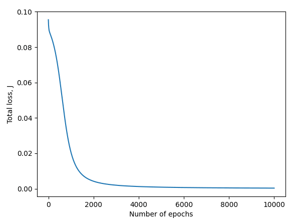
After 10,000 epochs, the total loss J of our neural network should reduce, leading to an improvement in prediction accuracy.

In a perfect scenario, plotting the total loss J against the number of iterations performed will reveal something like this:

Total loss J vs Number of epochs

With this sort of outcome, our trained neural network should do pretty well at predicting outputs that are very close to the expected outputs. For example:

x1 x2 y ao1
0 0 0 0.04
0 1 1 0.98
1 0 1 0.98
1 1 1 1.00

If we find the total loss J has not reduced at all or sufficiently after training, further optimisation may be achieved by experimenting with different learning rates α\alpha (e.g. 0.1, 0.01, 0.001). That's another topic in its own right...

Summary

Congratulations if you made it to the end and thanks for reading!

Here's what we covered, some in more detail than others:

  • Forward propagation
  • Sigmoid activation function
  • Concept of loss L and total loss J
  • Backpropagation using partial derivatives and the chain rule
  • Training to minimise the total loss J

Please comment below if you found this post useful or if you've spotted an error.

Top comments (0)