
Data science is gaining an ever more prominent role in production pipelines across the tech scene, and it’s clear why. Data scientists provide product teams with data modeling and analysis systems that provide valuable feedback on gathered data to improve the product. In the world of Big Data, data modeling and analysis is essential to the growth and success of businesses in almost every sector.
Data science by itself is only a support role. It provides data and findings in an understandable manner. So, how do we turn this process from a supportive role to a proactive, problem-solving one? This is where applied data science comes in. If you are a data scientist interested in the cloud or predictive model services for product teams, you’re in the right place.
Today, we’ll learn about the role of applied data science in tech. We’ll discuss the popular tools you’ll need as an applied data scientist, namely PySpark and serverless functions in Google Cloud and AWS. We’ll then build a scalable cloud model pipeline.
This article assumes the reader has experience with Python and data science. Take a look at the basics before continuing here.
Today, we’ll cover:
- What is applied data science?
- Serverless functions and data science
- AWS Serverless functions: Lambda
- Google Cloud Functions: Google’s serverless functions
- Introducing model pipelines
- PySpark for batch pipelines
- PySpark tutorial for applied data science
- What to learn next?
What is applied data science?
Applied data science is the process of using data science principles to answer business questions and create scalable systems that make product predictions based on past data.
The main difference between data science and applied data science is where their expertise ends. Both data scientists and applied data scientists focus on tracking data trends and creating visualizations. But applied data scientists go beyond this to focus on real-life applications that advise businesses on what to do with their findings.
Applied data science exists at the intersection of machine learning (ML) engineering and data science. Applied data scientists focus on building data products that product teams can integrate. For example, an applied scientist at a game publisher might build a recommendation service that different game teams can integrate into their products. Typically, this role is part of a central team that is responsible for owning a data product.
What is applied data science used for?
Applied data science is used to create forward-looking problem-solving programs through the use of machine learning systems. These systems take in masses of big data and use predictive analytics to draw conclusions for the future. Machine learning systems can even see trends too subtle for a human data scientist.
Well-designed ML data analytics programs are also scalable, meaning the work of a single applied data scientist can be widely adopted to benefit multiple product teams.
Data-driven predictions allow teams to take preemptive choices to maximize profit where they normally couldn’t. For example, an applied data scientist could create a program that tracks behavior on your subscription-based site, such as time per session, visits per week, etc. to predict when a subscriber was about to cancel their subscription.
Responding to this, the product team could send the subscriber a special deal or promotion to entice them to stay subscribed. Without applied data science, this prediction could not have been found, and the team could not act preemptively to keep its customer.
Tools of applied data science
Applied data scientists use many different tools to accomplish their varied responsibilities. Below, take a quick look at each and what role it takes in the process:
Python:
Python is the most widely used programming language for data science. Thanks to its massive libraries filled with data manipulation functions, flexibility, and relative ease of learning, Python has quickly become the industry standard. Common environments to work in are simple text editors, notebooks, or remote notebook environments like Amazon’s EC2.
Jupyter Notebooks:
Project Jupyter is a non-profit organization focused on making highly shareable open-source environments across different coding languages. Many data scientists use Jupyter notebooks as their choice of Python environment because of how effective it is for quickly downloading and using data from anywhere in the world. Sharing notebooks and data is very easy with Jupyter. This allows data scientists to share findings and methods to collectively push the capabilities of data science.
Kaggle:
Kaggle is an online collection of public data sets and notebooks discovered and shared by other data scientists. Kaggle’s goal is to increase the availability of discovered data science techniques and big data as a shared resource for all data scientists. It can be interfaced directly with Jupyter to import data and has resources to help with Pandas, Machine Learning, Deep learning and more.
BigQuery:
BigQuery is a serverless, scalable online warehouse of big data sets which can be used in code by placing queries in your Python code. The difference between Kaggle and BigQuery is that Kaggle contains programs created by data scientists and the data they used while BigQuery simply contains masses of data. The advantage of querying data is that it allows you to use the data without having to download and store such large collections on your local machine.
Pandas:
Pandas is a software library written for Python that contains extra structures and operations for data manipulation and analysis. This is particularly useful for data scientists as Pandas specializes in manipulating numerical tables and time series, which are common data forms in the data science world. Pandas also acts as a mediary for calling large datasets from internet collections like Kaggle and BigQuery.
PySpark and Apache Spark:
PySpark is the Python API to support Apache Spark. Apache Spark is a distributed framework that is designed to handle big data analysis. Spark acts as a large computational engine which can process huge sets of data through parallel processing and batch systems. By using these outsourced systems, data science teams can gain the use of a distributed framework without the need for expensive engineering teams and hardware.
Cloud Platforms: AWS, Azure, and GCP:
One of the reasons applied data scientists can create such scalable solutions is the active use of cloud computing technologies like Amazon AWS and Google’s Google Cloud Platform. These platforms give applied data scientists access to auto-scaling capabilities and heaps of big data too cumbersome to store on local drives.
Now, let's learn more about cloud computing’s most beneficial technology for data scientists: serverless functions.
Serverless functions and data science
Serverless functions are a prime tool for applied data scientists. They are a type of software that runs in a hosted environment maintained by a cloud-computing company like Amazon or Google.
Serverless functions are set up to respond to certain events, like an HTTP request, and respond with a programmed response, such as sending data packets. There are two main environments for working with serverless functions: AWS Lambda and Google Platform Cloud Functions. We will discuss each of them below
Benefits of serverless functions
Serverless functions are used by data scientists because these functions are very scalable. With serverless technologies, the cloud provider manages server provisioning, scales up machines, manages load balancers, and handles versioning.
Shifting these responsibilities to the cloud provider allows data scientists to focus less on operational concerns and be more active in DevOps. It also allows a single data scientist’s solution to be scaled massively without the need for an infrastructure team’s help.
AWS serverless functions: Lambda
AWS Lambda is a serverless computing service, or FaaS (Function as a Service), provided by Amazon Web Services. It is one of the most popular serverless computing services because it can be used alongside many programming languages, and it can handle an unlimited number of functions per project.
Lambda supports a wide array of potential triggers, including incoming HTTP requests, messages from a queue, customer emails, changes to database records, and much more.
How to create an echo function in AWS Lambda
An echo function is a simple AWS function that returns the content of the trigger event sent to the program. This is commonly used in applied data science to test and debug systems by tracking what event is triggering the system. With a simple echo program, a data scientist can determine at what stage a bug is occurring or if the event trigger is received and processed correctly.
This example will use Databricks Community Edition, a free notebook environment for use with AWS, GCP, PySpark, and more. You can download this at the Databricks website to follow along with all our examples to come.
Below we’ll create this function using AWS Lambda. To follow along, complete the following steps on your version of Databricks:
- Under “Find Services,” select “Lambda.”
- Select “Create Function.”
- Use “Author from scratch.”
- Assign a name (e.g. echo).
- Select a Python runtime.
- Click “Create Function.”
After running these steps, Lambda generates a file called lambda_function.py. The file defines a function called lambda_handler, which we’ll use to implement the echo service.
We’ll make a small change to this file, as shown below, so it will repeat the contents of the msg trigger sent to it.
def lambda_handler(event, context):

return {
        'statusCode': 200,
        'body': event['msg']
    }
Click “Save” to deploy the function, and then click “Test” to test the file. If you use the default test parameters, an error will be returned when running the function because no msg key is available in the event object. Click on “Configure test event”, and define the following configuration:
{
  "msg": "Hello from Lambda!"
}
Now our simple echo function is running on AWS Lambda. Thanks to the auto-scaling of AWS, we can trust that this will meet any level of demand and requires no monitoring.
Simple Storage Service (S3)
Simple Storage Service (S3) is a storage layer provided by AWS and a widely popular feature of this cloud service. S3 acts as a huge, durable hash table stored in the cloud that can host anything from individual files for websites to millions of files for data lakes.
Though AWS offers many other storage solutions, S3 is the most popular. All S3 data lies within the same “data lake”, meaning there are no hardware barriers between one company’s data and another's.
By changing permissions, a data scientist can give or gain access to any other data stored on S3. S3’s ease of sharing data and its durability make this tool an essential part of a data scientist’s life.
Below we’ll explore the basics of using S3 for data science in production. In order to use S3 to store our function to deploy, we’ll need a new S3 bucket, a policy for accessing it, and credentials for setting up command line access. Buckets on S3 are analogous to GCS buckets in GCP.
Let’s learn how to set up a bucket, define a user, and provide that user access to our bucket:
How to set up an S3 bucket:
S3 uses a multi-tiered system to order and pair data within the larger data lake. The first tier is a project, which can be thought of as an overarching folder to contain all lower elements. One user can have multiple projects on their account. After that, projects are broken into buckets that act as subfolders to hold related or cooperating objects and functions together.
Each account can, by default, make up to 100 buckets, and each bucket can hold up to 100 items. Buckets cannot be transferred between accounts but can be provisioned to other users through access points.
To set up a bucket, browse to the AWS console and select “S3” under find services. Next, select “Create Bucket” to set up a location for storing files on S3. Create a unique name for the S3 bucket, as shown in the figure below, and click “Next”. Finally, click “Create Bucket” to finalize setting up the bucket.

How to define a user in S3:
Before our bucket can be accessed, we need to create a user that can be granted permission.
In the AWS console, select “IAM” under “Find Services”. Next, click “Users” and then “Add user” to set up a new user. Create a username, and select “Programmatic access,” as shown below:

How to provide user access to an S3 bucket:
The next step is to provide that user with full access to our S3 bucket. First, use the “Attach existing policies option” and search for S3 policies to find and select the AmazonS3FullAccess policy, as shown in the figure below. Click “Next” to continue the process until a new user is defined.
At the end of this process, a set of credentials will be displayed, including an access key ID and secret access key. Store these values in a safe location.

Finally, we have to run the aws configure and aws s3 ls commands to test that the user credentials have appropriate permissions:
aws configure
aws s3 ls
Now our S3 bucket is all set up and has command line access! You will know if all is functioning as expected if the results include the name of the S3 bucket we set up at the beginning of this section.
More AWS concepts to learn:
You now have a good foundation to learn more about AWS Lambda functions and capabilities. Here are some topics to consider tackling next to keep your AWS learning going:
- Predictive model functions in Lambda
- Defining API gateways using Lambda
- Defining Lambda dependencies
Google Cloud Functions: Google’s serverless functions
For applied data scientists, the other main serverless environment used is Google Cloud Platform, where we can create Cloud Functions that operate much like Lambda from above. GCP is a good starter platform, as it is similar to standard Python development.
That being said, GCP has several drawbacks, such as:
- No elastic cloud storage
- Storage is not intuitive as Cloud Functions are read-only, with users only able to write to the
\tmpdirectory - Using spaces instead of indents for formatting can cause large-scale problems
- Less responsive support teams for issues
- Overly wordy documentation and APIs
Many developers agree that it’s best to design GCP code around later using it in Python’s Flask, as this allows you to leverage the advantages of GCP while also having access to elastic cloud storage.
How to create an echo service in GCP
Below we’ll create another echo service, this time in GCP. GCP provides a web interface for authoring Cloud Functions. This UI offers options for setting up a function’s triggers, specifying requirements for a Python function, and authoring the implementation of a Flask function. Let’s see how it’s done.
Setting up our environment:
First, we’ll set up our environment by doing the following:
- Search for “Cloud Function.”
- Click on “Create Function.”
- Select “HTTP” as the trigger.
- Select “Allow unauthenticated invocations.”
- Select “Inline Editor” for source code.
- Select Python 3.7 as the runtime.
- Write the name of your function in “Function to execute.”

After performing these steps, the UI will provide tabs for the main.py and requirements.txt files. The requirements file is where we will specify libraries, such as flask >= 1.1.1, and the main file is where we’ll implement our function behavior.
Deploying our function:
Now that we have our environment set up, we can start working on our program. We’re going to create a simple echo function that parses out the msg parameter from the passed-in request and returns this parameter as a JSON response. To use the jsonify function, we need to first include the flask library in the requirements.txt file.
The requirements.txt file and main.py files for the simple echo function are both shown in the snippet below.
# requirements.txt
flask

#main.py
def echo(request):
    from flask import jsonify

    data = {"success": False}
    params = request.get_json()

    if "msg" in params:
        data["response"] = str(params['msg'])
        data["success"] = True

    return jsonify(data)
Testing our function:
Now, click on the function name in the console and then click on the “Testing” tab to check if the deployment of the function worked as intended.
You can specify a JSON object to pass to the function and invoke the function by clicking “Test the function”, as shown in the figure below.
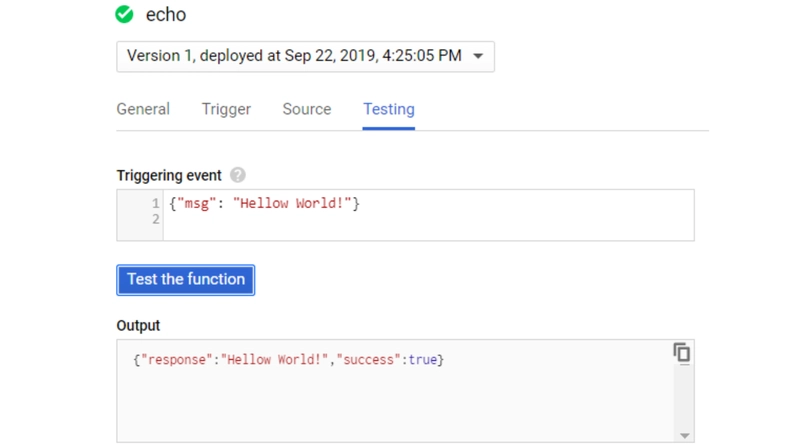
The result of this test is the JSON object returned in the Output dialog, which shows that invoking the echo function worked correctly.
Testing HTTP calls:
Now that the function is deployed and we have enabled unauthenticated access to the function, we can call the function over the web using Python. To get the URL of the function, click on the “trigger” tab. We can then use the requests library to pass a JSON object to the serverless function, as shown in the snippet below.
import requests

result = requests.post(
        "https://us-central1-gameanalytics.cloudfunctions.net/echo"
                    ,json = { 'msg': 'Hello from Cloud Function' })
print(result.json())
The result of running this script is aJSON payload that is returned from the serverless function. The output from the call is the JSON shown below:
{
    'response': 'Hello from Cloud Function',
    'success': True
}
Google Cloud Storage (GCS)
Google Cloud Storage is another cloud storage software that works similarly to AWS S3. S3 beats GCS in both latency and affordability. However, GCS supports significantly higher download throughput.

Below we’ll see how GCS can be used to create a bucket and save a file. We’ll also learn how to download a model file from GCS.
While GCP does provide a UI for interacting with GCS, we’ll explore the command line interface in this lesson since this approach is useful for building automated workflows.
Installing GCS libraries:
In order to interact with Cloud Storage using Python, we’ll also need to install the GCS library using the command shown below:
pip install --user google-cloud-storage
export GOOGLE_APPLICATION_CREDENTIALS=dsdemo.json
How to create a bucket in GCS:
Before we can store a file, we need to set up a bucket on GCS. We’ll create a bucket name called dsp_model_store where we’ll store model objects. The script below shows how to create a new bucket using the create_bucket function and how to iterate through all of the available buckets using the list_buckets function.
You’ll need to change the bucket_name variable to something unique before running this script.
from google.cloud import storage
bucket_name = "dsp_model_store"

storage_client = storage.Client()
storage_client.create_bucket(bucket_name)

for bucket in storage_client.list_buckets():
    print(bucket.name)
How to save a file in GCS:
To save the file to GCS, we need to assign a path to the destination, shown by the bucket.blob command below. We then select a local file to upload, which is passed to the upload function.
from google.cloud import storage

bucket_name = "dsp_model_store"
storage_client = storage.Client()
bucket = storage_client.get_bucket(bucket_name)

blob = bucket.blob("serverless/logit/v1")
blob.upload_from_filename("logit.pkl")
How to download from GCS:
The code snippet below shows how to download the model file from GCS to local storage. We download the model file to the local path of local_logit.pkl and then load the model by calling pickle.load with this path.
import pickle
from google.cloud import storage

bucket_name = "dsp_model_store"
storage_client = storage.Client()
bucket = storage_client.get_bucket(bucket_name)

blob = bucket.blob("serverless/logit/v1")
blob.download_to_filename("local_logit.pkl")
model = pickle.load(open("local_logit.pkl", 'rb'))
model
We can now store model files to GCS using Python and also retrieve them, enabling us to load model files in Cloud Functions.
More GCP topics to learn next:
With these two examples under your belt, you’re ready to seek more advanced GCP topics, such as:
- Predictive Cloud Functions
- Setting up Karas Models in Cloud Functions
- Cybersecurity through Access Management
- Dynamic models in Cloud Functions
Now we have a grasp on one of the main tools used by applied data scientists: serverless functions. Let’s move on to another popular concept necessary for understanding data science in production: the batch model pipeline and PySpark.
Introducing model pipelines
Pipelines are an essential piece for implementing machine learning programs. Machine learning can be thought of as simply the culmination of many steps of computation to decide a behavior or prediction. These steps of computation are split into chunks based on role to make them more modular and easier to design.
For example, one chunk may act as a filter to parse out all invalid data types, while another may sort the data based on a certain attribute. These chunks can be visualized as pipe segments.
When put back together, all data feeding into a machine learning program passes through these pipe segments in sequence, forming a model pipeline.
What are batch model pipelines?
Model pipelines can either have stream or batch processing. Stream model pipelines send data through their sequence as it is received and draw conclusions in real time. Batch model pipelines instead gather and manipulate data sets over a period of time and then pass them into the pipeline in a batch. The data is not acted on immediately and instead is stored for later use by another system.
Stream model pipelines are best suited for real-time applications, like analyzing social media reception during a press release. One downside of the stream model pipeline is that it can be temporarily thrown off by high-variance data, meaning its predictions can be erratic.
Batch model pipelines are best suited for processing large quantities of data when real-time results are not needed, like analyzing old sales reports to predict sales for next year’s summer season.
This prediction will not be used right away but will be by a marketing ML program when planning next year's campaigns. In this example, we can see the storage endpoint of batch model pipelines in action.
What tools do we use for batch model pipelines?
So, batch model pipelines involve processing lots of data at once, so we need a tool adept at mass data processing. There are several tools available for this sort of work, such as PySpark, Apache Airflow, Luigi, MLflow, and Pentaho Kettle.
PySpark has emerged as the preferred tool for data scientist’s batch model pipelines because of its unique specialty in working with large collections of data.
PySpark for batch pipelines
As a reminder, PySpark is the Python version of Apache Spark. Spark uses a distributed framework of machines to provide extremely quick computations regardless of data size.
This speed is largely due to Sparks core resilient distributed datasets (RDD) component. By allowing clusters of machines to simultaneously on processing a data set, RDD allows Spark to be both fault-tolerant and efficient. It also allows data scientists to build more scalable models as the same Spark-enabled model could handle anywhere from 10 to over 100,000 data points without any changes needed.
PySpark best practices
While PySpark is a very similar environment to Python, it has some unique best practices. Here are some best practices to keep in mind as you keep learning to maximize your PySpark effectiveness:
Avoid Dictionaries:
Using Python data types such as dictionaries means that the code might not be executable in a distributed mode. Instead, create another that can be used as a filter for a data set.
Limit Panda Usage:
Calling toPandas will cause all data to be loaded into memory on the driver node and prevents operations from being performed in a distributed mode. Do not use this command with large data set.
Avoid Loops:
Use group by and apply instead of loops to ensure your code is supported by execution environments down the line.
Minimize Pulling from Data frames:
Avoid operations that pull from a data set to memory. This will ensure your code is scalable to larger data sets that cannot download or fit easily onto local machines.
Use SQL:
SQL queries are easier to understand than some Pandas operations. Using SQL will allow your code to be more easily understood by other data scientists.
Now that we’ve learned some best practices, let's apply them in our first PySpark program!
PySpark tutorial for applied data science
One of the quickest ways to get up and running with PySpark is to use a hosted notebook environment.
Databricks is the largest Spark vendor and provides a free version for getting started called Community Edition.
The first step is to create a login on the Databricks website for the community edition. Next, perform the following steps to spin up a test cluster after logging in:
- Click on “Clusters” on the left navigation bar.
- Click “Create Cluster”.
- Assign a name, “DSP”.
- Select the most recent runtime (non-beta).
- Click “Create Cluster”.
- After a few minutes, we’ll have a cluster set up that we can use for submitting Spark commands.
For this example, we’ll be using a data set of NFL player’s performance in CSV format. To import this data, enter the following command:
stats_df = spark.read.csv("s3://dsp-ch6/csv/game_skater_stats.csv", header=True, inferSchema=True)
display(stats_df)
PySpark file formats
When using S3 or other data lakes, Spark supports a variety of different file formats for persisting data.
Parquet is the industry standard when working with Spark, but we’ll also explore Avro, ORC, and CSV. Avro is the best format for streaming data pipelines, while ORC is useful when working with legacy data pipelines.
To show the range of data formats supported by Spark, we’ll take the stats dataset and write it to Avro, then Parquet, then ORC, and finally CSV. After performing this round trip of data IO, we’ll end up with our initial Spark data frame.
Let's begin!
Avro
Avro is a distributed file format that is record-based. Parquet and ORC formats are column based. To start, we’ll save the stats data set in Avro format using the code snippet shown below:
# AVRO write
avro_path = "s3://dsp-ch6/avro/game_skater_stats/"
stats_df.write.mode('overwrite').format("com.databricks.spark.avro").save(avro_path)

# AVRO read
avro_df = sqlContext.read.format("com.databricks.spark.avro").load(avro_path)
This code writes the data set to S3 in Avro format using the Databricks Avro writer and then reads in the results using the same library. The result of performing these steps is that we now have a Spark data frame pointing to the Avro files on S3. Since PySpark lazily evaluates operations, the Avro files are not pulled to the Spark cluster until an output needs to be created from this dataset.
Parquet
Parquet on S3 is currently the standard approach for building data lakes on AWS, and tools such as Delta Lake are leveraging this format to provide highly-scalable data platforms. Parquet is a columnar-oriented file format that is designed for efficient reads when only a subset of columns are being accessed for an operation, such as when using Spark SQL.
Parquet is a native format for Spark, which means that PySpark has built-in functions for both reading and writing files in this format.
An example of writing the stats data frame as Parquet files and reading the result as a new data frame is shown in the snippet below.
# parquet out
parquet_path = "s3a://dsp-ch6/games-parquet/"
avro_df.write.mode('overwrite').parquet(parquet_path)

# parquet in
parquet_df = sqlContext.read.parquet(parquet_path)
In this example, we haven’t set a partition key, but as with Avro, the data frame will be split up into multiple files in order to support highly-performant read and write operations. When working with large-scale datasets, it’s useful to set partition keys for the file export using the repartition function.
ORC
ORC is another columnar format that works well with Spark. ORC's main benefit over Parquet is that it can support improved compression at the cost of additional compute cost. I’m including it in this chapter because some legacy systems still use this format.
An example of writing the stats data frame to ORC and reading the results back into a Spark data frame is shown in the snippet below.
# orc out
orc_path = "s3a://dsp-ch6/games-orc/"
parquet_df.write.mode('overwrite').orc(orc_path)

# orc in
orc_df = sqlContext.read.orc(orc_path)
CSV
To complete our round trip of file formats, we’ll write the results back to S3 in the CSV format.
To make sure that we write a single file rather than a batch of files, we’ll use the coalesce command to collect the data to a single node before exporting it. This is a command that will fail with large datasets, and in general, it’s best to avoid using the CSV format when using Spark. However, CSV files are still a common format for sharing data, so it’s useful to understand how to export to this format.
# CSV out
csv_path = "s3a://dsp-ch6/games-csv-out/"
orc_df.coalesce(1).write.mode('overwrite').format(
 "com.databricks.spark.csv").option("header","true").save(csv_path)

# and CSV read to finish the round trip
csv_df = spark.read.csv(csv_path, header=True, inferSchema=True)
Now that we’ve returned our file to CSV format, you’ve completed your first taste of PySpark as well as a tour of each of the file types.
What to learn next?
Congratulations! You’ve just learned how to use three of the most important tools for an applied data scientist: AWS (Lambda and S3), GCP (GCF and GCS), and PySpark. With these tools, we can build serverless functions, call functions through HTTP triggers, and also easily analyze big data. These tools have a lot of exciting features yet to explore, such as:
- Streaming model workflows
- Containers for reproducible models
- Models as web endpoints
- Prototype models
Educative’s course Data Science in Production: Building Scalable Model Pipelines walks you through each of these topics and more with added professional insights gained from the author’s years of experience in game development at Zynga. Learn hands-on with more code-based tutorials like those above and develop the skills recruiters are looking for in tomorrow’s data scientists.
Continue reading about data science on Educative
- Data Analysis Made Simple: Python Pandas Tutorial
- A Quick AWS Tutorial: the services you should definitely use
- Pandas Cheat Sheet: top 35 commands and operations
Start a discussion
Which of these tools that we went over is your preferred tool? Was this article helpful? Let us know in the comments below!

Oldest comments (0)