After blindly attempting to train the classifier (as seen in Part 2), I had a good long hard think about all the variables and all the possible combinations of things I could try and tweak to get results out of my naive Bayes classifier. I also had a good long hard think about how I would measure those results. What are good results? This is an important thing to consider in machine learning. You may think that accuracy is all that matters — but that’s not the case.
In this experiment, we’re attempting to classify observations into one of 34 different bins. If we look only at accuracy, we see only part of the picture. We can’t answer questions such as “is one category often misclassified as another category?” or “how many different categories does the classifier bin things into?” These questions have answers that are helpful in “debugging” our classifier, i.e. determining why it’s classifying things the way it is, and how we can improve our data and strategy in order to improve its accuracy. This is why confusion matrices are useful tools for visualizing the result of classification. Confusion matrices explain the how the errors in classification are distributed among the possible classes, shedding light on the overall behavior of the classifier.
If you’ll recall, our dataset class distribution looks like this:
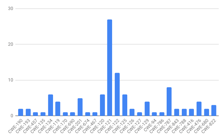
The labels are heavily skewed toward CWE-121. A classifier could achieve high accuracy in this dataset by simply guessing CWE-121 for every observation. This is a type of overfitting. If the data does not have a lot of descriptive power, i.e. the features I’ve chosen to extract from the binaries are not related to the CWE classes, I would expect the classifier to have this behavior.
To validate this, I made the decision to perform a trial where I trained the classifier on the dataset, but randomized the labels. This trial provides a baseline that can be inspected to compare subsequent, properly trained trials to in order to differentiate their results from random noise.
With this in mind, I also identified a few different parameters to tweak in order to potentially improve classifier performance. We can perform classification at the basic block level or at the binary level. We can also choose to use a threshold to discard “uninformative” basic blocks, as described in the previous post. In addition, there is more than one naive Bayes classifier variant. Both Bernoulli naive Bayes and multinomial naive Bayes are applicable classifiers for our data. Finally, we can represent our features in two different ways: we can use a boolean representation for each opcode in each basic block, i.e. whether or not that opcode was present, or we can use an integer, i.e. how many times that opcode was present in the block. I attempted to exercise a reasonable combination of these parameters when training and evaluating the classifier.
Throughout the rest of this post, you will see results for three separate classifiers; one a Bernoulli naive Bayes classifier trained on the binary-featured dataset, one a multinomial naive Bayes classifier trained on the binary-featured dataset, and one a multinomial naive Bayes classifier trained on the integer-featured (also referred to as “event-featured”) dataset.
Tuning The Threshold
As a refresher, in the previous post I talked about a clever way we could use the probability estimates returned by naive Bayes to identify basic blocks that are common across many CWE classes vs. those that are unique to a CWE class. The idea is that if the classifier thinks each of the classes is equally likely for a block, then that block is not informative for classification and can be discarded. Conversely, if the classifier is very confident that a block belongs to a particular class, then it is informative and should be kept.
If we’re going to use this idea to discard basic blocks, we first need a way to measure this difference in probabilities between the classes. I chose to use the difference between the highest probability class and lowest probability class returned by the classifier. If the difference is small, the distribution is relatively even across the classes — if the difference is large, it is likely to be uneven. Semi-formally:
m=x_highest — x_lowest
Now that we have a metric, we need to know at what value blocks become “informative” vs. “uninformative.” In other words, we need to know what our threshold is. A good way to determine this is by training the classifier and seeing how classification performs with respect to different threshold values. This is a type of classifier tuning similar to that done by K-nearest Neighbors when choosing a value for K. This type of tuning requires a validation data set.
Typically, when training a classifier, you need at least two datasets: a training data set, with which to train your classifier, and a testing dataset, to evaluate your classifier’s accuracy on. But when you want to test your trained classifier in under different conditions and pick the best condition as a parameter of your classifier, you need an additional dataset called a validation set in order to maintain the independence of the testing data from the process of training. Otherwise, you risk overfitting your classifier to your data, and will likely produce results in your experiment that translate poorly to unseen data.
To tune the threshold, I trained each of the three classifiers on their respective data and plotted their accuracy with respect to different threshold values. I created two plots — one where the accuracy was calculated with respect to basic block level classification, and one where the accuracy was calculated by having the “informative” basic blocks “vote” on what they believed the binary they came from should be labeled as.

Accuracy curve with respect to threshold for each naive Bayes classifier applied to basic blocks
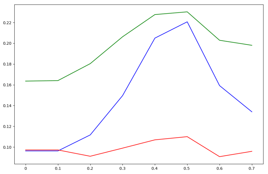
Accuracy curve with respect to threshold for each naive Bayes classifier applied to binaries
The accuracy curve per basic block looks kind of like garbage — each of the classifiers performs fairly differently. However, when voting is applied to classify whole binaries, we see each classifier’s accuracy peaks at a threshold value of about 0.5. Therefore, we choose this as our threshold value for each classifier.
Also, for fun, I plotted the distribution of the threshold metric. If I’m right about some basic blocks being common to all the CWE classes and others being unique, we should see a bimodal distribution of this metric.
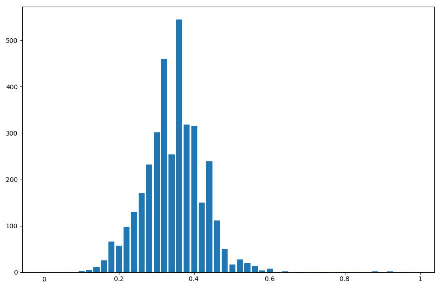
Threshold metric distribution for Bernoulli naive Bayes on binary-featured dataset

Threshold metric distribution for multinomial naive Bayes on binary-featured dataset

Threshold metric distribution for multinomial naive Bayes on integer-featured dataset
The bimodal distribution hypothesis holds, if only barely. It’s not very pronounced, but it can be seen in each of the three distributions. This is useful information to have, because we could have chosen other metrics by which to create a threshold. It’s possible that another metric would plot a more emphatic bimodal distrbution. Likely such a metric would perform better as a threshold.
Calculating The Baseline
The next thing to do is calculate the accuracy and confusion matrices for the baseline trial with the labels in the dataset randomized. I calculated this for each of the three classifiers, and each returned a very similar confusion matrix. One is shown below.

An example confusion matrix produced from random noise baseline testing
You’ll notice that the classifier is classifying nearly everything as CWE-121, which is exactly as expected. We’ll try to improve on this overfitting with our different training strategies.
The accuracy of each classifier under different conditions was also pretty similar between classifiers in the random trials. To calculate these accuracies, twenty trials were run. The data was randomized differently for each trial and split into training, validation, and testing datasets containing 1/3 of the data each.
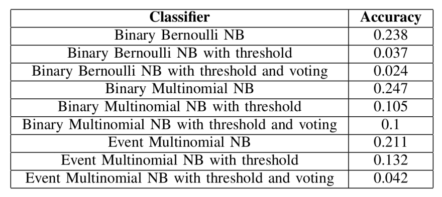
Baseline accuracies for the different classifiers, trained on randomly labeled data
Unsurprisingly, using a threshold on the randomly labeled data reduces the accuracy by an enormous amount. And while it’s not shown here, it’s also worth noting that using a threshold on this data reduces the dataset by a significant amount. We expect more of the data to be preserved during normal trials.
Training The Classifiers
Finally we’re ready to evaluate our classifiers on real data with some different parameters. I evaluated each classifier under three different conditions — first, training and testing for basic block classification without any threshold value, second, basic block classification with a threshold value of 0.5, and third, whole binary classification with a threshold value of 0.5 using the basic blocks to vote on a label for their binary.
Each of these conditions were tested with twenty trials of randomized data, training/validation/testing split of 1/3 of the dataset for each. The results for each of the three classifiers are shown below.

Bernoulli naive Bayes accuracy on binary-featured dataset

Multinomial naive Bayes accuracy on binary-featured dataset
Multinomial naive Bayes accuracy on integer-featured dataset
The first thing you’ll notice is that the accuracy of each of the classifiers at basic block classification is lower than the random noise. This seems like a bad sign, but it is also odd. Any sort of significant deviation from the random baseline implies that the classifier is picking some kind of pattern out of the data. We turn to the confusion matrices to try to diagnose the difference between the random baseline and the actual run.

Confusion matrix for Bernoulli naive Bayes applied to binary-featured dataset for basic block classification
While the random baseline classifier overfit to CWE-121, there is some evidence here that our properly-trained naive Bayes classifier does not overfit as strongly. In particular, CWE-119 and CWE-416 are guessed quite often as well. In addition, we are able to correctly classify a significant number of blocks from CWE-416 and CWE-122, in addition to CWE-121. Unfortunately, this also causes many CWE-121 basic blocks to be incorrectly guessed as other classes. Realizing that this is likely due to the poor labeling of the dataset, it seems we can say that there is some predictive value in the opcode features extracted from the basic blocks, though there’s too much noise for the classifier to produce an acceptable accuracy.
The other unfortunate observation about the classifier accuracies is that applying a threshold does not increase the accuracy of the classifier. In the best case, it only reduces it by about 0.01 — which is a marked improvement over the baseline, but not terribly helpful. Voting even further decreases the accuracy, debunking the theory that we can use the probability outputs from naive Bayes for whittling down the list of informative basic blocks.
The takeaways
As with all good science, just because something doesn’t work out the way you want or expect it to, doesn’t mean there isn’t a reason. I looked through the documentation for the naive Bayes classifier implementation I used from scikit-learn, attempting to find something to help me gain some insight into the probability outputs, and ran across this lovely gem:
![]()
That's a note from sckit-learn.org about naive Bayes classifiers.
…so the idea of using the probabilities is fundamentally flawed, and in order to implement this, I need to use another classifier. Back to the drawing board. However, this experiment hasn’t been a waste. I’ve learned valuable information about my data composition, and eliminated a possible classifier from the list of candidates. Better, I learned that the data does have some informative value! Next up is identifying an appropriate replacement classifier and continuing the research.

Latest comments (0)