
Logistic regression is the bread-and-butter algorithm for machine learning classification. If you’re a practicing or aspiring data scientist, you’ll want to know the ins and outs of how to use it. Also, Scikit-learn’s LogisticRegression is spitting out warnings about changing the default solver, so this is a great time to learn when to use which solver. 😀
FutureWarning: Default solver will be changed to 'lbfgs' in 0.22.
Specify a solver to silence this warning.
In this article, you’ll learn about Scikit-learn LogisticRegression solver choices and see two evaluations of them. Also, you’ll see key API options and get answers to frequently asked questions. By the end of the article, you’ll know more about logistic regression in Scikit-learn and not sweat the solver stuff. 😓
I’m using Scikit-learn version 0.21.3 in this analysis.
When to use Logistic Regression
A classification problem is one in which you try to predict discrete outcomes, such as whether someone has a disease. In contrast, a regression problem is one in which you are trying to predict a value of a continuous variable, such as the sale price of a home. Although logistic regression has regression in its name, it’s an algorithm for classification problems.
Logistic regression is probably the most important supervised learning classification method. It’s a fast, versatile extension of a generalized linear model.
Logistic regression makes an excellent baseline algorithm. It works well when the relationship between the features and the target aren’t too complex.
Logistic regression produces feature weights that are generally interpretable, which makes it especially useful when you need to be able to explain the reasons for a decision. This interpretability often comes in handy — for example, with lenders who need to justify their loan decisions.
There is no closed-form solution for logistic regression problems. This is fine — we don’t use the closed form solution for linear regression problems because it’s slow.
Solving logistic regression is an optimization problem. Thankfully, nice folks have created several solver algorithms we can use. 😁
Logistic regression is a primary algorithm to use for most classification problems. It's a fast, versatile extension of a generalized linear model. It produces feature weights that are generally interpretable, which makes it especially useful when you need to be able to explain the reasons for a decision. This interpretability often comes in handy — for example, with loan denials.
There is no closed-form solution for logistic regression. This is fine, because we don't even use the closed form solution to solve linear regression problems because it's slow. Instead, solving logistic regression is an optimization problem. Thankfully, very nice folks have created several algorithms to solve it. 😁
Solver Options
Scikit-learn ships with five different solvers. Each solver tries to find the parameter weights that minimize a cost function. Here are the five options:
-
newton-cg— A newton method. Newton methods use an exact Hessian matrix. It's slow for large datasets, because it computes the second derivatives. -
lbfgs— Stands for Limited-memory Broyden–Fletcher–Goldfarb–Shanno. It approximates the second derivative matrix updates with gradient evaluations. It stores only the last few updates, so it saves memory. It isn't super fast with large data sets. It will be the default solver as of Scikit-learn version 0.22.0. -
liblinear— Library for Large Linear Classification. Uses a coordinate descent algorithm. Coordinate descent is based on minimizing a multivariate function by solving univariate optimization problems in a loop. In other words, it moves toward the minimum in one direction at a time. It is the default solver prior to v0.22.0. It performs pretty well with high dimensionality. It does have a number of drawbacks. It can get stuck, is unable to run in parallel, and can only solve multi-class logistic regression with one-vs.-rest. -
sag— Stochastic Average Gradient descent. A variation of gradient descent and incremental aggregated gradient approaches that uses a random sample of previous gradient values. Fast for big datasets. -
saga— Extension of sag that also allows for L1 regularization. Should generally train faster than sag.
An excellent discussion of the different options can be found in this Stack Overflow answer.
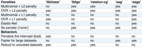
The chart below from the Scikit-learn documentation lists characteristics of the solvers, including the the regularization penalties available.
Why is the Default Solver Being Changed?
liblinear is fast with small datasets, but has problems with saddle points and can't be parallelized over multiple processor cores. It can only use one-vs.-rest to solve multi-class problems. It also penalizes the intercept, which isn't good for interpretation.
lbfgs avoids these drawbacks, is relatively fast, and doesn't require similarly-scaled data. It's the best choice for most cases without a really large dataset. Some discussion of why the default was changed is in this GitHub issue.
Let's evaluate the Logistic Regression solvers with two prediction classification projects — one binary and one multi-class.
Solver Tests
Binary classification solver example
First, let's look at a binary classification problem. I used the built-in scikit-learn breast_cancer dataset. The goal is to predict whether a breast mass is cancerous.

The features consist of numeric data about cell nuclei. They were computed from digitized images of biopsies. The dataset contains 569 observations and 30 numeric features. I split the dataset into training and test sets and conducted a grid search on the training set with each different solver. You can access my Jupyter notebook used in all analyses at Kaggle.
The most relevant code snippet is below.
solver_list = ['liblinear', 'newton-cg', 'lbfgs', 'sag', 'saga']
params = dict(solver=solver_list)
log_reg = LogisticRegression(C=1, n_jobs=-1, random_state=34)
clf = GridSearchCV(log_reg, params, cv=5)
clf.fit(X_train, y_train)
scores = clf.cv_results_['mean_test_score']

for score, solver in zip(scores, solver_list):
    print(f"  {solver} {score:.3f}" )
liblinear 0.939
newton-cg 0.939
lbfgs 0.934
sag 0.911
saga 0.904
The values for sag and saga lag behind their peers.
After scaling the features, the solvers all perform better and sag and saga are just as accurate as the other solvers.
liblinear 0.960
newton-cg 0.962
lbfgs 0.962
sag 0.962
saga 0.962
Now let's look at an example with three classes.
Multi-class solver example
I evaluated the logistic regression solvers in a multi-class classification problem with Scikit-learn's wine dataset. The dataset contains 178 samples and 13 numeric features. The goal is to predict the type of grapes used to make the wine from the chemical features of the wine.
solver_list = ['liblinear', 'newton-cg', 'lbfgs', 'sag', 'saga']
parameters = dict(solver=solver_list)
lr = LogisticRegression(random_state=34, multi_class="auto", n_jobs=-1, C=1)
clf = GridSearchCV(lr, parameters, cv=5)
clf.fit(X_train, y_train)
scores = clf.cv_results_['mean_test_score']

for score, solver, in zip(scores, solver_list):
    print(f"{solver}: {score:.3f}")
liblinear: 0.962
newton-cg: 0.947
lbfgs: 0.955
sag: 0.699
saga: 0.662
Scikit-learn gives a warning that the sag and saga models did not converge. In other words, they never arrived at a minimum point. Unsurprisingly, the results aren't so great for those solvers.
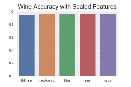
Let's make a little bar chart using the Seaborn library to show the differences for this problem.

After scaling the features between 0 and 1, then sag and saga reach the same mean accuracy scores as the other models.
liblinear: 0.955
newton-cg: 0.970
lbfgs: 0.970
sag: 0.970
saga: 0.970
Note the caveat that both of these examples are with small datasets. Also, we're not looking at memory and speed requirements in these examples.
Bottom line: the forthcoming default lbfgs solver is a good first choice for most cases. If you're dealing with a large dataset or want to apply L1 regularization, I suggest you start with saga. Remember that saga needs the features to be on a similar scale.
Do you have a use case for newton-cg or sag? If so, please share in the comments. 💬
Next, I'll demystify key parameter options for LogisticRegression in Scikit-learn.

Parameters
The Scikit-learn LogisticRegression class can take the following arguments.
penalty, dual, tol, C, fit_intercept, intercept_scaling, class_weight, random_state, solver, max_iter, verbose, warm_start, n_jobs, l1_ratio
I won't include all of the parameters below, just excerpts from those parameters most likely to be valuable to most folks. See the docs for those that are omitted. I've added additional information in italics.
C — float, optional, default = 1
Smaller values have more regularization. Inverse of regularization strength. Must be positive value. Usually search logarithmically: [.001, .01, .1, 1, 10, 100, 1000]
random_state : int, RandomState instance or None, optional (default=None) Note that you must set the random state here for reproducibility.
solver {‘newton-cg’, ‘lbfgs’, ‘liblinear’, ‘sag’, ‘saga’}, optional (default=’liblinear’). See the chart above for more info.
Changed in version 0.20: Default will change from ‘liblinear’ to ‘lbfgs’ in 0.22.
multi_class : str, {‘ovr’, ‘multinomial’, ‘auto’}, optional (default=’ovr’)
If the option chosen is ‘ovr’, then a binary problem is fit for each label. For ‘multinomial’ the loss minimised is the multinomial loss fit across the entire probability distribution, even when the data is binary. ‘multinomial’ is unavailable when solver=’liblinear’. ‘auto’ selects ‘ovr’ if the data is binary, or if solver=’liblinear’, and otherwise selects ‘multinomial’.
Changed in version 0.20: Default will change from ‘ovr’ to ‘auto’ in 0.22. ovr stands for one vs. rest. See further discussion below.
l1_ratio : float or None, optional (default=None)
The Elastic-Net mixing parameter, with 0 <= l1_ratio <= 1. Only used if penalty='elasticnet'. Setting `l1_ratio=0 is equivalent to using penalty='l2', while setting l1_ratio=1 is equivalent to using penalty='l1'. For 0 < l1_ratio <1, the penalty is a combination of L1 and L2. Only for saga.
Commentary:
If you have a multiclass problem, then setting multi-class to auto will use the multinomial option every time it's available. That's the most theoretically sound choice. auto will soon be the default.
Use l1_ratio if want to use some L1 regularization with the saga solver. Note that like the ElasticNet linear regression option, you can use a mix of L1 and L2 penalization.
Also note that an L2 regularization of C=1 is applied by default.
After fitting the model the attributes are: classes_, coef_, intercept_, and n_iter. coef_ contains an array of the feature weights and intercept_ contains an
Logistic Regression FAQ:
Now let's address those nagging questions you might have about Logistic Regression in Scikit-learn.
Can I use LogisticRegression for a multilabel problem — meaning one output can be a member of multiple classes at once?
Nope. Sorry, if you need that, find another classification algorithm here.
Which kind of regularization should I use?
Regularization shifts your model toward the bias side of things in the bias/variance tradeoff. Regularization makes for a more generalizable logistic regression model, especially in cases with few data points. You're going to want hyperparameter search over the regularization parameter C.
If you want to do some dimensionality reduction through regularization, use L1 regularization. L1 regularization is Manhattan or Taxicab regularization. L2 regularization is Euclidian regularization and generally performs better in generalized linear regression problems.
You must use the saga solver if you want to apply a mix of L1 and L2 regularization. The liblinear solver requires you to have regularization. However, you could just make C such as a large value that it had a very, very small regularization penalty. Again, C is currently set to 1 by default.
Should I scale the features?
If using sag and saga solvers, make sure the features are on a similar scale. We saw the importance of this above.

Should I remove outliers?
Probably. Removing outliers will generally improve model performance. Standardizing the inputs would also reduce outliers' effects.
RobustScaler can scale features and you can avoid dropping outliers. See my article discussing scaling and standardizing here.
Which other assumptions really matter?
Observations should be independent of each other.
Should I transform my features using polynomials and interactions?
Just as in linear regression, you can use higher order polynomials and interactions. This transformation allows your model to learn a more complex decision boundary. Then, you aren't limited to a linear decision boundary. However, overfitting becomes a risk and interpreting feature importances gets trickier. It might also be more difficult for the solver to find the global minimum.

Should I do dimensionality reduction if there are lots of features?
Probably. Principal Components Analysis is a nice choice if interpretability isn't vital. Recursive Feature Elimination can help you remove the least important features. Alternatively, L1 regularization can drive less important feature weights to zero if you are using the saga solver.
Is multicollinearity in my features a problem?
It is for interpretation of the feature importances. You can't rely on the model weights to be meaningful when there is high correlation between the variables. Credit for effecting the outcome variable might go to just one of the correlated features.
There are many ways to test for multicollinearity. See Kraha et al. (2012) here.
One popular option is to check the Variance Inflation Factor (VIF). A VIF cutoff around 5 to 10 is usually as problematic, but there's a lively debate as to what an appropriate VIF cutoff should be.
You can compute the VIF by taking the correlation matrix, inverting it, and taking the values on the diagonal for each feature.
The correlation coefficients alone are not sufficient to determine problematic multicollinearity with multiple features.
If the sample size is small, getting more data might be most helpful for removing multi-collinearity.
When should I use LogisticRegressionCV?
[LogisticRegressionCV](https://scikit-learn.org/stable/modules/linear_model.html) is the Scikit-learn algorithm you want if you have a lot of data and want to speed up your calculations while doing cross-validation to tune your hyperparameters.
Wrap
Now you know what to do when you see the LogisticRegression solver warning — and better yet, how to avoid it in the first place. No more sweat! 😅
I suggest you use the upcoming default lbgfs solver for most cases. If you have a lot of data or need L1 regularization, try saga. Make sure you scale your features if you're using saga.
I hope you found this discussion of logistic regression helpful. If you did, please share it on your favorite social media so other people can find it, too. 👏
I write about Python, Docker, data science, and more. If any of that’s of interest to you, read more here and sign up for my email list.😄


Happy logisticing!


Top comments (0)