The Normal and Binomial distributions, explained with Python

(Originally published on darrendube.com).

The Binomial and Normal (or Gaussian) distributions are some of the most common distributions in Statistics. They are used anywhere from predicting movements in stock prices, to grading SAT tests. As an introduction to data visualisation in python, we will be plotting a binomial distribution, then plotting a normal estimation to the binomial.

(If you've only come for the visualisation part, skip to this point)

What are the Normal and Binomial Distributions

Even if you didn’t take a high school statistics class, you’ve probably still encountered the Gaussian (or normal) distribution in a math or science class.

If you created a histogram to represent the heights of people in a class, it would likely create a bell curve, with the more common heights in the middle, and the less common ones on the sides.

If you increased the number of subjects in your sample, the graph would more and more closely resemble the shape of a normal distribution:

The probability distribution function of a normal distribution is :

The shape of the graph is determined by its mean and standard deviation. The graph is centred around the mean, and the standard deviation determines how stretched it is in the x-direction.

Besides the heights of people in a class, many other random variables follow the normal distributions, including measurement error, SAT scores, and shoe sizes. The area under two points on the graph, divided by the area of the whole graph, gives the probability of a value between those two points.

Closely related is the binomial distribution. Even if you haven’t heard of it, it is very intuitive to understand.

Consider a coin toss: the probability of hitting either heads or tails is $0.5$ . If there is a fixed number of trials, the binomial distribution is used to calculate the probability of, e.g., getting $2$ heads in $10$ tries. It is represented by the probability density function:

meaning, in $n$ trials, each with a probability $p$ of success, the probability of getting $x$ successes is $P_{x}$ . In the coin toss example, $n=10$ , $p=0.5$ , and success means getting heads. While it is possible that there will be no heads in all 10 trials, it is unlikely, hence $P_{0}$ will be extremely low. Likewise, it is unlikely all 10 tosses will be heads, hence $P_{10}$ will likely be low too. The more likely number of successes would be in the middle, with the most likely being $n\times p (=10)$ .

If you increase the number of trials, the shape of the graph starts to look very familiar...

If the number of attempts is large enough, the binomial distribution resembles a normal distribution. This means a normal distribution can be used to estimate the binomial by using $\mu=np$ and $\sigma=np(1-p)$ . This is very useful when, for instance, you're trying to find the probability it takes more than 30 tries when $n=100$ (which would normally require you to find $P_{x}$ for every number from 31-100).

However, there's a catch: the binomial distribution deals with discrete variables (i.e. there is no $P_{8.443}$ or $P_{3.142}$ , only whole numbers), whereas the normal distribution deals with continuous variables. This means the normal distribution is only an approximation to the binomial.

I realise this is by no means an exhaustive introduction. If you're still confused, this and this are more in-depth explanations.

Plotting the binomial distribution

We can plot a graph of the probabilities associated with each number of tries. In this example, I’ll be using Python and matplotlib.

If you do not have matplotlib installed on Python yet, install it by typing pip install matplotlib.

Begin by importing matplotlib and math. We'll need math to get the value of $e$ , and the $nCx$ function.

import math
import matplotlib.pyplot as pyplot

Firstly, we need to define the probability density function of the binomial distribution. To recall:

In python:

def binomial(x, n, p):
    return math.comb(n, x) * (p ** x) * ((1 - p) ** (n - x))

In this case, to make the binomial distribution more clearly resemble a normal distribution, I will make $n$ equal to $50$ . $p$ will be 0.5. We also need to initialise a list to store the 50 values we get from the binomial p.d.f for each value of $x$ , and another list to store keys (that basically number each value of $x$ in the previous list).

n = 50
p = 0.5
binomial_list = []
keys = []

Now that we have initialised all the variables we need, we can now iterate over each number from $1$ to $50$ to get values of $P_{x}$ for each, and we need to fill the keys[] list with numbers from $1$ to $50$ :

for x in range(50):
    binomial_list.append(binomial(x, n, p))

for y in range(50):
    keys.append(y)

All that's left is to plot the graph!

pyplot.bar(x=keys, height=binomial_list)
pyplot.show()

And voila!

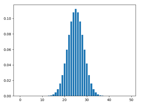
As you can see, it clearly resembles a normal distribution. To see if it actually has the shape of a normal distribution, we can superimpose the normal curve by inserting this code (before the pyplot.show() expression:

def normal_distribution(x, mu, sigma):
    return (math.exp(-0.5 * ((x - mu) / sigma) ** 2)) / (sigma * math.sqrt(2 * math.pi))

pyplot.plot(keys, [normal_distribution(y, n*p, math.sqrt(n*p*(1-p))) for y in range(50)])

(Originally published on darrendube.com).