
What is a Time-Travel Query?
Imagine a database that never forgets, no matter what you throw at it. A place for unbiased facts where all changes are tracked. Now imagine you are roped into an adventure with a crazy data science robot. He puts you in the bSQL time-travel mobile and takes you on a trip down data lane.
You learn that application data is always evolving as values are added and removed from the database. Through rich record histories, you find yourself accessing a new dimension of data by exploring its evolution over time.
Enhanced visibility is perhaps one of the most powerful features of bSQL and allows us to answer important questions like: What was this value before I updated it? When did this value get deleted? How does the history of my data affect the current state?
bSQL allows you to access the history of your data by writing special “time-travel” queries.
Financial Data Example
In the financial demo database there are two containers.
companies keeps track of the company metadata such as name, sector, and symbol.
pricing keeps track of the current stock prices.
Ever row in pricing references a row in companies. Every time the share price changes an AMEND statement is sent to the pricing container to make the corresponding updates. Logical right.
Querying from the pricing container using a basic SELECT statement reads from the current state of the system. Using our Multi-Version Database, we can run analytics on previous events. In the bSQL language this involves using the LIFETIME keyword to query from the lifetime of the container.
For a full description of the financial database check out the bSQL docs here.
Understanding the Lifetime Query
SELECT symbol, price, timestamp
   FROM LIFETIME financial.pricing;
The above query uses the LIFETIME keyword to query from the entire record history of the pricing container. The following output is produced:
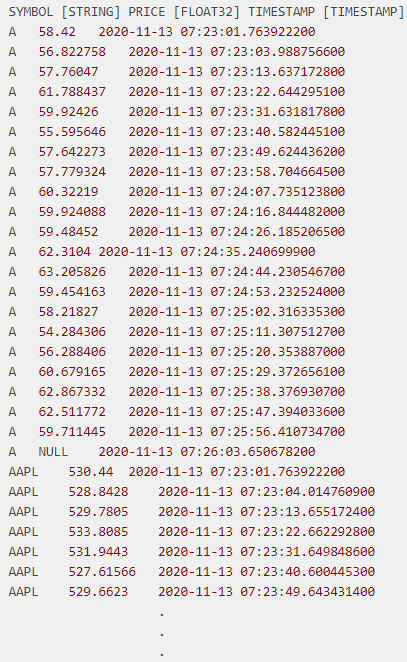
It is important to notice a couple of things here:
The output is sorted by the primary key of the container, the symbol column.
The records associated with the primary key are ordered by the time the mutation was made in ascending order.
The first entry of the group represents when the record was inserted into the container.
Subsequent entries represent when values were either updated using the
AMMENDcommand or removed from the current state using theDISCONTINUEcommand.When a record is removed from the current state of the container using a
DISCONTINUEcommand, a tombstone record is added to the data.
Let’s look at the record history of the symbol A. When the record was introduced into the container the price was 58.42. The records that follow it show how the price was updated. The final record with a NULL price value, represents a tombstone record. This means that A was removed with the DISCONTINUE command from the current state of the database at 2020–11–13 07:26:03.650678200.

Discontinued Data
Although it sounds paradoxical, let’s search for deleted data. Here we will use the DISCONTINUED keyword to filter our previous query.
SELECT *
     FROM LIFETIME financial.pricing
  WHERE DISCONTINUED(pricing);
The corresponding output is:
SYMBOL    PRICE   ...    52_WEEK_HIGH       TIMESTAMP
A         NULL    ...    NULL       2020–11–13 07:26:03.650678200
MMM       NULL    ...    NULL       2020–11–13 07:26:03.670677500
When a DISCONTINUE statement is run, a tombstone record is inserted into the target container. Time-travel queries allow us to access the tombstones displayed above. As you can see, the primary key, in this case both MMM and A, as well as any timestamp column is preserved in the tombstone. This allows us to embed such statements in more complex queries and preserve discontinued data.
Joining and Aggregating Histories
Now let’s look at how we can use the LIFETIME keyword to gain insight into the history of our data.
SELECT c.name, COUNT(*) AS number_of_versions, AVG(p.price)
    FROM LIFETIME financial.pricing AS p
       JOIN financial.companies AS c
       ON c.symbol = p.symbol
    GROUP BY name
FILTER 10;
Let’s break down this query:
The complete history of pricing is joined with the current state of companies to retrieve the name metadata.
The records are then grouped by the
namecolumn and theCOUNTandAVGfunctions are applied. This will return the number of versions of each primary key, as well as the average price over these versions respectively.The output is limited to be the first 10 records.
This query returns:
C.NAME           NUMBER_OF_VERSIONS             AVG(P.PRICE)
3M Co.           22                             133.92297224564985
ACE Limited      21                             103.51996685209728
AES Corp         21                             18.495395614987327
AFLAC Inc        21                             70.05538577125186
AGL Resources Inc. 21                           56.701499938964844
AMETEK Inc       21                             59.99528685070219
AT&T Inc         21                             25.695445378621418
AbbVie Inc.      21                             57.20997020176479
Abbott Laboratories 21                          45.31997081211635
Accenture        21                             89.67997051420666
The number of versions tells us the number of INSERT, AMEND, and DISCONTINUE statements that were run on each record. While other companies where changed 21 times, 3M Co. was changed 22 times, this makes sense because 3M Co. was discontinued from the data set, adding the “discontinued” version. We were able to compute the average price across all versions regardless of whether or not the record existed in the current state.
Using the Timestamp Column
Let’s see what we can uncover using the timestamp column.
SELECT symbol, MAX(p.price) AS max_price, MIN(p.price) AS min_price,
   MAX(p.timestamp) - MIN(p.timestamp) AS life_span
     FROM LIFETIME financial.pricing AS p
   GROUP BY p.symbol
  ORDER BY life_span DESC
FILTER 10;
Let’s take a deeper look at this query.
The complete history of pricing is grouped by the symbol column. We compute the min_price, max_price, and the time since the record was inserted and when it was last amended or discontinued as life_span.
We ordered the output by the life_span.
We limited the number of outputs to be the first 10 records.
SYMBOL          MAX_PRICE         MIN_PRICE           LIFE_SPAN
VLO             52.99             40.63915            182
VMC             68.85             56.499134           182
ZMH             98.06             84.10976            182
VIAB            88.27             75.919136           182
YUM             77.16             63.209763           182
XYL             38.64             24.689758           182
VFC             61.71059          51.781025           182
XRAY            46.86             32.909756           182
XOM             94.99             81.03975            182
V               225.89061         215.96103           182
Our output produces an interesting dataset that gives us the amount of time between the first insertion and the last mutation in seconds. The dataset we produced allows us to analyze how the life span of a stock affects other target variables. As you can see, the bSQL language allows you to compute rich datasets that leverage the power of an immutable database.
Conclusion
If you made it this far, hats off to you Sherlock Codes! We are always working on more bSQL features and will continue to post. Our goal at blockpoint is to provide you with with insightful tools to get the most out of immutable databases. Please leave any comments or suggestions down below.


Top comments (0)