
Performance engineering is a big deal when you’re serving millions of users from every corner of the globe. We previously wrote about a large engineering transformation program for Jira & Confluence, which we codenamed Vertigo – read more about the overall program here.
As part of the Vertigo program, we knew we were going to have to invest a lot of engineering effort into performance, and in particular the performance of Jira. While we have always spent time over the years improving Jira’s performance using the tools and architecture at-hand, the Vertigo architecture brought a host of new opportunities to further improve the performance and reliability of Jira.
Now it’s time to share some of the work we did during the Vertigo program to improve Jira’s performance on the new platform. It’s not just about the gains we achieved, but how we rethought some of our old strategies (such as caching data in application memory) to be successful on a new underlying architecture that required different approaches.
The new capabilities unlocked by running Jira in the cloud on AWS allowed us to make substantial performance & reliability gains. While we were proud of the improvements we have been able to make so far, we know there is more work to be done to improve the performance of Jira cloud. We see performance as an ongoing journey and are continuing to invest substantial effort into all aspects of Jira’s performance.
Betting big on zero affinity
One of the goals of the Vertigo architecture was to achieve “zero affinity”. This meant that incoming requests could be served by any Jira application node running behind a load balancer. There are numerous benefits of this architecture, and zero affinity is one of the concepts included in the widely used 12-Factor Application model.
From a performance perspective, one of the key benefits of zero affinity is the ability to horizontally scale up the number of application nodes processing requests in response to increased load. This means that we are much better able to handle larger Jira customers on our infrastructure, and was one of the key enablers of our ability to increase the maximum license tier for Jira Cloud from 2,000 to 5,000 users.
In Jira Server, and our previous Jira Cloud architecture (codenamed Unicorn), frequently used customer data was cached in-memory across requests, this provided a substantial performance benefit, because cached data could be accessed in microseconds. However, our heavy reliance on in-memory caching also came with problems, in particular as data sizes grew too large to be feasibly kept in the in-memory cache, which could sometimes lead to a performance cliff.
To allow us to move to a zero affinity architecture, we now have to remove all of these long-lived in-memory caches from within the Jira application nodes. This introduced performance challenges because data that could previously be looked up in microseconds now had to be fetched from a remote database. To address our performance challenges, we adopted a number of patterns:
- For data that needs to be re-used during the progress of a request, keep it in an in-memory request-scoped cache
- For data that is re-usable across requests and was expensive to compute, we would store it in Memcached
- For data that existed in the database, we would focus on changing our queries to make more efficient usage of our Postgres database
Challenges in data access patterns
We started our journey towards zero affinity by first removing all in-memory cross-request caching. The cross-request caches were replaced with request-scoped caches kept in-memory on each Jira application node. This allowed us to make a single database call for information that was frequently used during a request, for example metadata about the current user. Once this work was completed we were able to investigate and understand where our performance problems were. What we expected to see was a performance degradation because the loss of cross-request caching meant that we had to talk to the database more frequently instead of reading data from in-memory stores.
A general pattern of challenges that we saw where what we called “n+1” access patterns, where we would first make a request to the database to fetch a list of objects, and would then make subsequent calls to fetch additional data one-by-one. For example, take the following example code snippet:
// Gets a list of Projects that are 'special'
Collection projects = projectManager.getAllProjects()
return projects.stream()

// Each call to #isSpecial calls the database
.filter(p -> specialProjectManager.isSpecial(p)).collect()
The above code demonstrates a typical pattern that was used extensively throughout the Jira codebase. Previously this was not a performance problem, because both ProjectManager and SpecialProjectManager would have implemented a caching layer that would allow them to generally return results based on in-memory data. When these caches changed from cross-request to request-scoped, we would see many caches no longer be effective, as they would be hit only once per request.
Going back to the above code example, we have to know a bit more information to determine the performance overhead:
- What is the overhead of calling the database?
- How big is the list of projects?
Under our architecture, we saw calls to the database typically take 0.5 – 2 ms of network time. The reason we had high network times was that we deployed our Jira application nodes in multiple availability zones, and we enabled high availability features on our RDS databases, this meant that we would often have to make cross-AZ requests in order to contact the database.
In addition to the network time, there was also query execution time on the database. For simple queries such as lookup by ID, we found that the network overhead was generally larger than the query time and that typically we expect a mean overall query time of 1 ms seen from the Jira application side.
As for the size of the project list, this is something that varied significantly between different customer sizes:
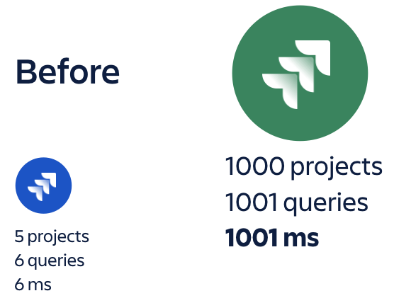
This shows how the performance overhead from the “n+1” data access pattern varied dramatically based on customer size. For small customers, the overhead was present, but not significant, while for larger customers the overhead became substantial.
Bulk loading of data
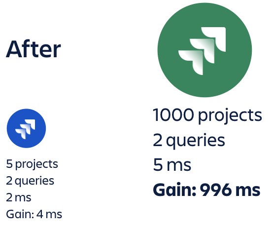
The fairly consistent pattern we applied to fix “n+1” data access patterns was to load data in bulk, by creating new methods that required only a single (or some constant number) of database calls. Taking the above example of loading special projects, this might now look like:
// Gets a list of Projects that are 'special'
Collection<Project> projects = projectManager.getAllProjects()

return specialProjectManager.filterSpecialProjects(projects)
The execution time of the new query might be slightly slower than previously, perhaps taking a few additional milliseconds. However, the overall performance improvement of the new approach would be substantial, particularly on customers with larger data sets.
This pattern of bulk loading worked very well. However, we saw a number of challenges in making these performance improvements:
- Finding the code path involved in the “n+1” was often difficult, as call paths could be distributed across many classes
- In some cases the amount of data being fetched from the DB was excessive (e.g., tens of thousands of rows), and we would have to use an alternative approach
- The surface area of “n+1” performance problems was very large, meaning that we had to find a clear way to prioritise the work.
Developing observability tools
To start to find performance problems on our new platform, we cloned the data from several internal instances and imported them onto the Vertigo platform. This provided us with a good data set to find codepaths that were causing bad performance.
Once we had identified that we could reproduce slow requests using these data sets, we had to determine how to take a slow request and map that to a root cause in code. We started by leveraging instrumentation from our database connection pool, Vibur DBCP, which allowed us to track all queries that were executed during a request. These queries were normalised and grouped together, and associated with measurements of connection acquisition time, query execution time, and result set processing time. This data was then sent via our logging pipeline to Splunk, where we built dashboards to provide both cross-request aggregation views and single request drill-downs.
These dashboards were very helpful in allowing us to see which requests were slow due to n+1 problems. However, the challenge we had was associating the queries with the code that was causing this performance issue. While it was fairly easy to find the store layer that performed the actual query, the code looping over method calls might be many layers removed.
In order to assist us in identifying the exact code causing large numbers of DB calls per request, we developed a tool that we called the DB Stack Trie. The idea was that we would capture the stack trace every time we accessed the database, and aggregate stack traces together into a weighted Trie data structure, with nodes representing the filename, line number and numbers of DB calls made, and edges representing where the call-stack branched. To help us visualise the breakdown of DB calls during a single request we created a Treemap.
An example of one generated Treemap is shown below, which was used during an investigation into how to speedup CSV issue export. This was a particularly extreme example, as the request required just over 90 thousand database calls!

Together, this tooling allowed us to identify high impact performance problems, and determine the root cause. We then refactored our code to utilise patterns such as bulk loading of data, or more effective queries that pushed computation into the database.
Improving application node performance
As we progressively made changes to improve the performance of our database access patterns, we saw the proportion of time taken in the database shrink. This was great progress, and we were very happy with the performance improvements that we saw, but the request times were still larger than we expected. To address this, we began a process of investigating potential performance bottlenecks that were present inside the Jira application, or on the hardware our application nodes were running on.
Splitting types of workloads
Initially, our Jira application was deployed as a homogeneous fleet on EC2, with each node in the autoscaling group having an identical configuration. This was a sub-optimal configuration because we had multiple types of workloads present in Jira:
- Inbound webserver requests (e.g. page loads, REST requests) that we wanted to respond to with low-latency
- Background tasks (e.g. sending emails and webhooks, or performing synchronisation with external systems) that had high throughput requirements, but less strict latency requirements
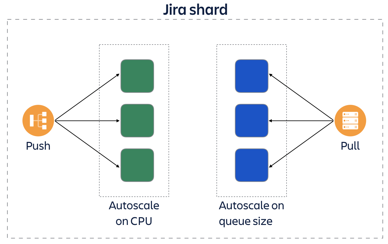
Because the same Jira application nodes were responsible for fulfilling both workloads, we were unable to tune our configuration to either specific use case. To address this problem we split our deployment into two groups that could autoscale independently:
- Webserver nodes that were optimised for low-latency response
- Worker nodes that were optimised for high throughput
Both webserver and Worker nodes would run the same code (but with different configuration parameters) and are deployed in parallel when changes are released.
The results of this split were very positive. By moving the background load from all Jira nodes to just the worker nodes and then optimising these nodes for throughput we were able to reduce the overall number of nodes needed to serve peak load by approximately 40%.
CPU profiling
The Jira webserver nodes were deployed on c4.4xlarge EC2 instances, and scaled up on CPU utilisation. This scaling rule was found based on experimentation, and we found that performance measurably degraded once the average CPU usage went above this threshold. This observation indicated:
- Our performance was most likely CPU bound, or alternatively bound to another resource that correlated with CPU
- If our application was indeed CPU bound, then would potentially expect to improve request latency by fixing CPU bottlenecks
We started investigating whether any non-CPU resources were creating performance bottlenecks, checking things such as network IO and disk IO. Our investigations indicated that there was no bottleneck on these resources, so that led us back to needing to investigate our CPU usage more deeply.
Flame Graphs
To investigate our CPU usage and get detailed insights into behaviour in production, we decided to utilise Java Flame graphs, as described by Netflix. These offered a number of benefits:
- This type of profiling adds a low overhead, meaning that we could utilise these in production
- The CPU profiles cover all code executing on the system, meaning that we can see if non-Java code is consuming CPU
We selected a few production Jira webserver nodes and run the Flame Graph profiles on them, and we got results that look similar to the following image:

What we immediately noticed was that __clock_gettime was taking up an unexpectedly large portion of the overall CPU. In addition, we notice that get time invocation is making a system call. To solve this, we investigated changing the clock source to a hardware supported source, in this case tsc (time stamp counter). For more information on clock sources, check out this article from redhat.
We started out by testing the clocksource change on nodes within a single autoscaling group, by running:
echo 'tsc' >
/sys/devices/system/clocksource/clocksource0/current\_clocksource
Following this we were able to re-run the Flame Graph to compare results:

The difference CPU usage from __cloud_gettime is dramatic when comparing the two Flame Graphs. We can also notice that the CPU usage of the Java code appears to have increased between the two Flame Graphs. This has occurred because the CPU usage change when we enabled the tsc clocksource was dramatic enough for our autoscaling rules to kick in and reduce the size of the autoscaling group.
It turns out others have found similar performance problems with the Xen clocksource, such as Brendan Gregg from Netflix who talked about this in 2014. In fact, this is now the default recommendation from AWS for modern instance classes.
Overly interrupted CPU cores
As part of our investigation into our CPU behaviour, we noticed that some CPU cores had higher usage than average. While this wouldn’t be that surprising if it were random and transient, what we observed was that cores 5 and 6 were consistently reporting higher utilisation across all Jira application nodes. The consistency suggested that there was an underlying root cause that led to these CPU cores being used more heavily.
On a hunch, we suspected that network interrupt behaviour could be causing this high utilisation of particular cores. While we had done significant amounts of work to reduce the number of DB calls per request, the Jira application is still quite chatty with the database, which will lead to a large number of network interrupts per-request. To get further information we checked
/proc/interrupts
What we saw was that two CPU cores were handling all the interrupts – and that these were CPUs 5 and 6!
So we had a likely potential cause for the unequal core utilisation of our CPUs, but now we had to figure out how to distribute the load more evenly. Luckily Linux has a feature called Received Packet Steering (RPS) that allows us to define how different CPU cores will handle incoming network packets. By default this is disabled, and the core receiving the network interrupt will also process the packet. In order to reduce load on CPUs 5 and 6, we tried setting the RPS configuration to direct incoming packet processing to all other CPUs. This approach worked as we had hoped, and successfully distributed our CPU utilisation in a more even manner.
EC2 C5 instances
In parallel to work investigating potential CPU bottlenecks, our team was also investigating using the new C5 instance class for EC2, which was released at AWS re:Invent 2017. The new instance class aimed to offer improved CPU performance and included a brand-new hypervisor called Nitro.
The Nitro hypervisor is based on the Linux KVM, and offered one feature that was particularly interesting to us – the kvmclock. At this stage, we were still investigating the approach we would take to consistently enable the tsc clock source and Received Packet Steering configuration in production, in order to address the above-discussed CPU bottlenecks.
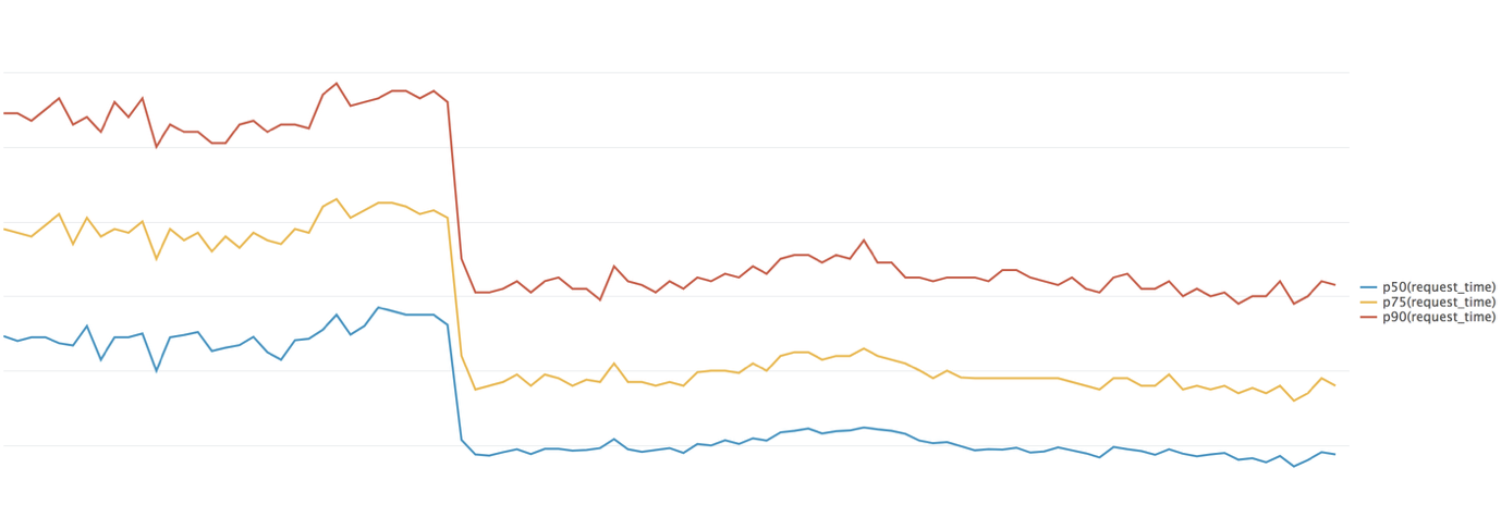
We first tested c5.4xlarge instances in our staging environment, then deployed them to one of our production environments to get some performance numbers. What we immediately saw was a substantial performance improvement in server response times across many different requests types. The following chart shows the performance change in server-side request latency for serving the Jira View Issue page, where we saw a drop of approximately 30% across the 50th, 75th and 90th percentiles.
Our monitoring also showed that on the C5 instance class the CPU load was now spread out evenly across available cores. To validate that our issue with interrupts being handled by a small number of CPUs was solved, we ran /proc/interrupts again. This showed that CPUs 3 through to 10 were handling network interrupts with approximately even distribution.
The journey continues!
The new Vertigo architecture produced a number of performance challenges, but also many more opportunities for us to improve the performance and reliability of Jira. By investing in observability tooling we were able to understand the performance of our system and make the changes necessary to get great performance improvements.
While we have come a long way in improving the performance of Jira Cloud, we know that we still have a lot of work to do to continue to improve performance. This blog has focussed on the work we have been doing in the Jira server to improve performance, but there have also been substantial efforts to improve the performance of our frontend.
In a future blog, we’ll talk further about other performance improvement streams, such as improving front-end performance for page loads, and how approached performance improvements that allowed Jira to scale better for our largest customers.
. . .
P.S. If you love sinking your teeth into juicy engineering problems like this, we’re hiring. Lots. Just sayin’.
The post Caching in: performance engineering in Jira Cloud appeared first on Work Life by Atlassian.


Top comments (0)