Introduction
Machine learning is explained in a single line is the set of rules that the system automatically generates to solve a problem based on certain patterns in the data. The machine learning problems can be classified into three main categories:
- Supervised Learning methods - both data and labels available
- Unsupervised Learning methods - only data and no labels
- Reinforcement Learning methods - Rewards and punishment-based systems mostly used in robotics
Machine learning models are greatly influenced by the features of our data.
Feature Engineering
All machine learning models take certain input and generate certain output which depends upon the type of problem at hand, it might be a float quantity if it is a regression problem or an integer representing the predicted class in case of classification or it can be a decision if it is a reinforcement learning problem.
The data that we feed into the machine learning models are nothing but features that ultimately decide the output. The better the features, the better the model performance.
Feature engineering refers to the selection of appropriate and important features for your machine learning models.
Possible problems with raw data:
Missing Data
Most ML algorithms can not work with missing data, it becomes necessary to deal with missing data before proceeding further, this calls for Data Cleaning which can be accomplished by either of the following strategies:
- Get rid of the missing features
dataFrame.dropna(inplace=True)
- Set the values to mean / median / mode The SimpleImputer can be very beneficial in this case
from sklearn.impute import SimpleImputer
computer = SimpleImputer(strategy="mean") # can be median or mode
imputer.fit(dataFrame)
Categorical data
The machine learning models deal with numerical values so it is often required to change your categorical data and encode it to numerical data. sklearn provides you with inbuilt methods to achieve this:
Ordinal Encoding
Ordinal Encoding provides the categories an encoded integer while preserving the ordinal nature of the variables:
from sklearn.preprocessing import OrdinalEncoder
ordinal_encoder = OrdinalEncoder()
encoded_dframe = ordinal_encoder.fit_transform(dataFrame)
One Hot Encoding
One Hot Encoding creates one binary attribute per category: one attribute equal to 1 when the category is "cold" for example and 0 otherwise and similarly 1 for "hot" and 0 otherwise and so on. This can be implemented by:
from sklearn.preprocessing import OneHotEncoder
cat_encoder = OneHotEncoder()
dframe_1hot = cat_encoder.fit_transform(dataFrame)
This produces a SciPy matrix instead of a NumPy array. This is very useful when we have categorical attributes with thousands of categories.
Unscaled Data
The data at hand is mostly on different scales for example in a dataset for housing price prediction, the number of rooms can range from 2-10 whereas the area can vary from 1000-5000. It is often found that scaled data performs better in machine learning.
Min Max Scaler
The MinMaxScaler is a transformer available in sklearn in which the numerical values are shifted and recalculated so that they range from 0 to 1. This is done simply by subtracting the min value and then dividing by the max minus min value. This is sometimes also called normalization.
Standard Scaler
Standardization first subtracts the mean value (so that the standardized values always have 0 mean) and then divides by the standard deviation (so that the resulting values have a unit standard deviation). Unlike min max scaler standard scaler does not bound the data to be on a specific scale. It is however less affected by the outliers.
from sklearn.preprocessing import StandardScaler
sc=StandardScaler()
dframe_std=sc.fit_transform(dataFrame)
Imbalanced Data
When the examples of a particular class are way too less as compared to the other class, this is a situation we call imbalanced data. It is important to have balanced data in order for the ML model to properly perform.
Imbalanced Data can be handled via one of the following techniques:
SMOTE (Synthetic Minority Oversampling Technique) – Oversampling
SMOTE (synthetic minority oversampling technique) is one of the most commonly used oversampling methods to solve the imbalance problem.
It aims to balance class distribution by randomly increasing minority class examples by replicating them.
SMOTE synthesizes new minority instances between existing minority instances. It generates virtual training records by linear interpolation for the minority class. These synthetic training records are generated by randomly selecting one or more of the k-nearest neighbors for each example in the minority class. After the oversampling process, the data is reconstructed and several classification models can be applied for the processed data.
from imblearn.over_sampling import SMOTE
oversample = SMOTE()
X, y = oversample.fit_resample(X, y)
SMOTEENN (A combination of over and under sampling)
SMOTE can generate noisy samples by interpolating new points between marginal outliers and inliers. This issue can be solved by cleaning the space resulting from over-sampling.
In this regard, Tomek’s link and edited nearest-neighbors are the two cleaning methods that have been added to the pipeline after applying SMOTE over-sampling to obtain a cleaner space. The two ready-to-use classes imbalanced-learn implements for combining over- and undersampling methods are (i) SMOTETomek and (ii) SMOTEENN.
from collections import Counter
from sklearn.datasets import make_classification
X, y = make_classification(n_samples=5000, n_features=2, n_informative=2,
...                            n_redundant=0, n_repeated=0, n_classes=3,
...                            n_clusters_per_class=1,
...                            weights=[0.01, 0.05, 0.94],
...                            class_sep=0.8, random_state=0)
print(sorted(Counter(y).items()))
[(0, 64), (1, 262), (2, 4674)]
from imblearn.combine import SMOTEENN
smote_enn = SMOTEENN(random_state=0)
X_resampled, y_resampled = smote_enn.fit_resample(X, y)
print(sorted(Counter(y_resampled).items()))
[(0, 4060), (1, 4381), (2, 3502)]
from imblearn.combine import SMOTETomek
smote_tomek = SMOTETomek(random_state=0)
X_resampled, y_resampled = smote_tomek.fit_resample(X, y)
print(sorted(Counter(y_resampled).items()))
[(0, 4499), (1, 4566), (2, 4413)]
SMOTEENN tends to clean more noisy samples than SMOTETomek.
Correlation in Data and Output
In regression problems, the correlation between certain features and the target variable can be beneficial. Sometimes a combination of one or more variables can better correlate with the target variable than individual variables. It is thus necessary to look for such patterns in the dataset.
Some feature selection that can be beneficial:
Feature selection can be very important and the selection of best features can reduce the computation power required in processing a lot of them, which can also help in less time complexity in certain algorithms.
Brute Force Correlation Processing
We manually calculate the correlation between various features and drop the ones that are more correlated than the predetermined threshold
Sample code on the Paribas-Cardif-Claim-Data can be (for code and dataset refer https://github.com/amartya-dev/feature_selection/blob/master/feature_selection.ipynb :
import numpy as np
import pandas as pd
import matplotlib.pyplot as plt
import seaborn as sns
from sklearn.model_selection import train_test_split
from sklearn.feature_selection import chi2
from sklearn.feature_selection import SelectKBest, SelectPercentile
from sklearn.feature_selection import mutual_info_classif, mutual_info_regression
from sklearn.feature_selection import SelectKBest, SelectPercentile
df = pd.read_csv('./dataset/Paribas-Cardif-Claim-Data/train.csv', nrows=50000)
print(df.shape)
print(df.head())
# Get Numerical features from dataset
numerics = ['int16', 'int32', 'int64', 'float16', 'float32', 'float64']
numerical_features = list(df.select_dtypes(include=numerics).columns)
data = df[numerical_features]
print("Dropping the non numeric data : ", data.shape, " is the shape")
print(data.head())
X = data.drop(['target', 'ID'], axis=1)
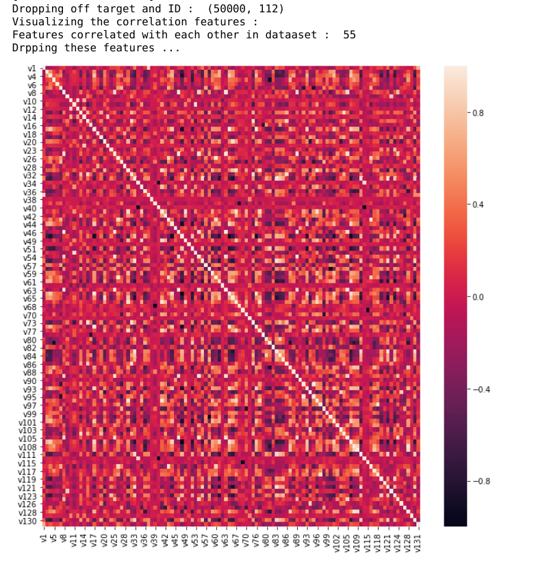
print("Dropping off target and ID : ", X.shape)
# Visualize Correlated Features
print("Visualizing the correlation features : ")
corr = X.corr()
fig, ax = plt.subplots()
fig.set_size_inches(11, 11)
sns.heatmap(corr)
# Brute Force Method to find Correlation between features
def correlation(data, threshold=None):
# Set of all names of correlated columns
col_corr = set()
corr_mat = data.corr()
for i in range(len(corr_mat.columns)):
for j in range(i):
if (abs(corr_mat.iloc[i, j]) > threshold):
colname = corr_mat.columns[i]
col_corr.add(colname)
return col_corr
correlated_features = correlation(data=X, threshold=0.8)
print("Features correlated with each other in dataaset : ", len(set(correlated_features)))
print("Drpping these features ...")
X.drop(labels=correlated_features, axis=1, inplace=True)
X.to_csv(r'./dataset/brute_force_corr_processed.csv')
The Output:
Highly correlated Feature Groups
Another method which is slightly better than the brute force correlation is creating feature groups from the data available and then further identify the best features in that group using a classifier such as the Random Forest Classifier:
df = pd.read_csv('./dataset/Paribas-Cardif-Claim-Data/train.csv', nrows=50000)
print(df.shape)
print(df.head())

# Get Numerical features from dataset
numerics = ['int16', 'int32', 'int64', 'float16', 'float32', 'float64']
numerical_features = list(df.select_dtypes(include=numerics).columns)
pd.options.mode.chained_assignment = None
data = df[numerical_features]
print("Dropping the non numeric data : ", data.shape, " is the shape")
print(data.head())

X = data.drop(['target', 'ID'], axis=1)
print("Dropping off target and ID : ", X.shape)

# Build a Dataframe with Correlation between Features
corr_matrix = X.corr()
# Take absolute values of correlated coefficients
corr_matrix = corr_matrix.abs().unstack()
corr_matrix = corr_matrix.sort_values(ascending=False)
# Take only features with correlation above threshold of 0.8
corr_matrix = corr_matrix[corr_matrix >= 0.8]
corr_matrix = corr_matrix[corr_matrix < 1]
corr_matrix = pd.DataFrame(corr_matrix).reset_index()
corr_matrix.columns = ['feature1', 'feature2', 'Correlation']
print("Correlation matrix \n : ", corr_matrix.head())

# Get groups of features that are correlated amongs themselves
grouped_features = []
correlated_groups = []

for feature in corr_matrix.feature1.unique():
    if feature not in grouped_features:
        # Find all features correlated to a single feature
        correlated_block = corr_matrix[corr_matrix.feature1 == feature]
        grouped_features = grouped_features + list(correlated_block.feature2.unique()) + [feature]

        # Append block of features to the list
        correlated_groups.append(correlated_block)

print('Found {} correlated feature groups'.format(len(correlated_groups)))
print('out of {} total features.'.format(X.shape[1]))

for group in correlated_groups:
    print(group)
    print('\n')

# Investigating features further within one group
group = correlated_groups[3]
print(group)

# Select features with less missing data
for features in list(group.feature2.unique()) + ['v17']:
    print(X[feature].isnull().sum())

print("Using Random forest classifier to find best features : ")
y = data['target']
y.shape
# Train Test Split
X_train, X_test, y_train, y_test = train_test_split(X, y, test_size=0.3, random_state=101)
print(X_train.shape, y_train.shape, X_test.shape, y_test.shape)

from sklearn.ensemble import RandomForestClassifier

features = list(group.feature2.unique()) + ['v17']
rfc = RandomForestClassifier(n_estimators=20, random_state=101, max_depth=4)
rfc.fit(X_train[features].fillna(0), y_train)

# Get Feature Importance using RFC
importance = pd.concat([pd.Series(features), pd.Series(rfc.feature_importances_)], axis=1)
importance.columns = ['feature', 'importance']
importance.sort_values(by='importance', ascending=False)

to_drop = set()
for i in ('v8', 'v105', 'v54', 'v63', 'v25', 'v89'):
    to_drop.add(i)

X_train.drop(labels=to_drop, axis=1, inplace=True)
X_test.drop(labels=to_drop, axis=1, inplace=True)

X = pd.merge(X_train, X_test)
X.to_csv(r'./dataset/Highly_corr_group_processed.csv')
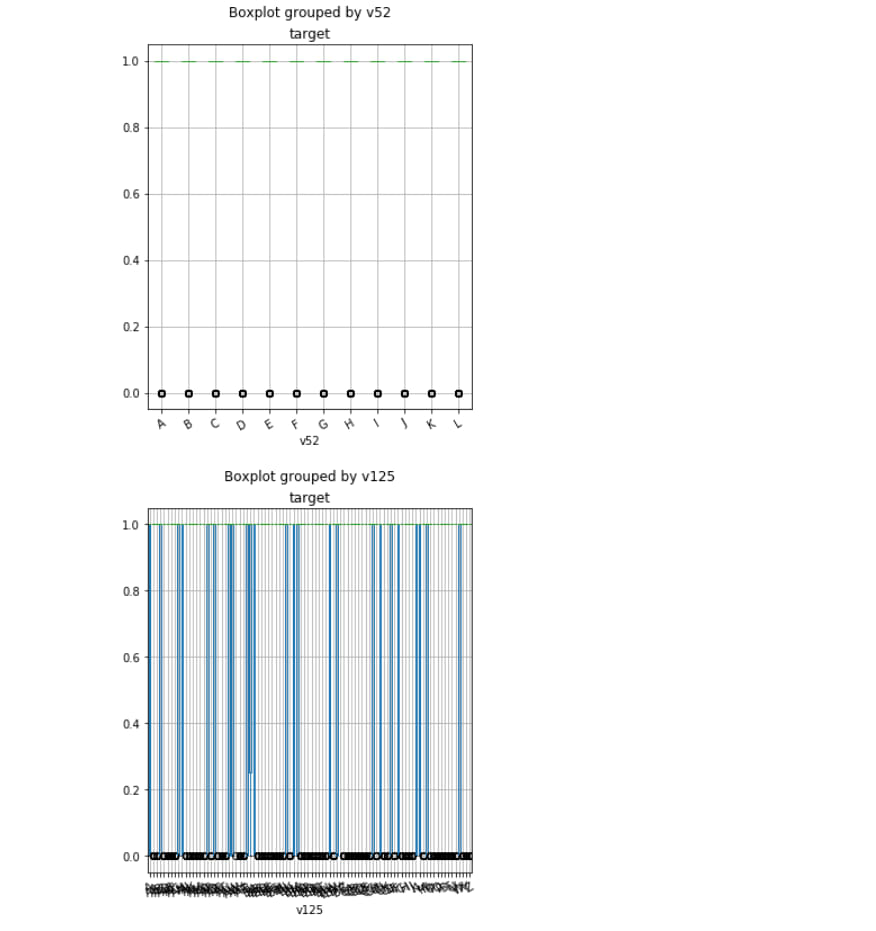
Fisher Score Chi-Squared
This is the measure of independent variables, we can use the fisher score in order to determine the best variable for the problem at hand. Sample code:
df = pd.read_csv('./dataset/Paribas-Cardif-Claim-Data/train.csv', nrows=50000)

df.boxplot('target', 'v75', rot=30, figsize=(5, 6))
df.boxplot('target', 'v52', rot=30, figsize=(5, 6))
df.boxplot('target', 'v125', rot=30, figsize=(5, 6))
df.boxplot('target', 'v91', rot=30, figsize=(5, 6))
df.boxplot('target', 'v107', rot=30, figsize=(5, 6))

print("\nGetting to know categorical data")

cat_df = df.select_dtypes(include=['object']).copy()

print(cat_df.head())

# Encode categorical variables into numbers
label1 = {k: i for i, k in enumerate(df['v3'].unique(), 0)}
label2 = {k: i for i, k in enumerate(df['v22'].unique(), 0)}
label3 = {k: i for i, k in enumerate(df['v24'].unique(), 0)}
label4 = {k: i for i, k in enumerate(df['v30'].unique(), 0)}
label5 = {k: i for i, k in enumerate(df['v31'].unique(), 0)}
label6 = {k: i for i, k in enumerate(df['v47'].unique(), 0)}
label7 = {k: i for i, k in enumerate(df['v52'].unique(), 0)}
label8 = {k: i for i, k in enumerate(df['v56'].unique(), 0)}
label9 = {k: i for i, k in enumerate(df['v66'].unique(), 0)}
label10 = {k: i for i, k in enumerate(df['v71'].unique(), 0)}
label11 = {k: i for i, k in enumerate(df['v74'].unique(), 0)}
label12 = {k: i for i, k in enumerate(df['v75'].unique(), 0)}
label13 = {k: i for i, k in enumerate(df['v79'].unique(), 0)}
label14 = {k: i for i, k in enumerate(df['v91'].unique(), 0)}
label15 = {k: i for i, k in enumerate(df['v107'].unique(), 0)}
label16 = {k: i for i, k in enumerate(df['v110'].unique(), 0)}
label17 = {k: i for i, k in enumerate(df['v112'].unique(), 0)}
label18 = {k: i for i, k in enumerate(df['v113'].unique(), 0)}
label19 = {k: i for i, k in enumerate(df['v125'].unique(), 0)}

df['v3'] = df['v3'].map(label1)
df['v22'] = df['v22'].map(label2)
df['v24'] = df['v24'].map(label3)
df['v30'] = df['v30'].map(label4)
df['v31'] = df['v31'].map(label5)
df['v47'] = df['v47'].map(label6)
df['v52'] = df['v52'].map(label7)
df['v56'] = df['v56'].map(label8)
df['v66'] = df['v66'].map(label9)
df['v71'] = df['v71'].map(label10)
df['v74'] = df['v74'].map(label11)
df['v75'] = df['v75'].map(label12)
df['v79'] = df['v79'].map(label13)
df['v91'] = df['v91'].map(label14)
df['v107'] = df['v107'].map(label15)
df['v110'] = df['v110'].map(label16)
df['v112'] = df['v112'].map(label17)
df['v113'] = df['v113'].map(label18)
df['v125'] = df['v125'].map(label19)

X = df[['v3', 'v22', 'v24', 'v30', 'v31', 'v47', 'v52', 'v56', 'v66', 'v71', 'v74', 'v75', 'v79', 'v91', 'v107', 'v110',
        'v112', 'v113', 'v125']]
print(X.head())

# Train Test Split
y = df['target']
y.shape
X_train, X_test, y_train, y_test = train_test_split(X, y, test_size=0.3, random_state=101)
X_train.shape, y_train.shape, X_test.shape, y_test.shape

# Calcualte the Fisher Score (chi2) between each feature and target
fisher_score = chi2(X_train.fillna(0), y_train)
fisher_score

p_values = pd.Series(fisher_score[1])
p_values.index = X_train.columns
p2 = p_values.sort_values(ascending=True)

print(p2.index[0], " is the most important feature here")

return (p2.index[0])
Output:


Please feel free to drop a message at Ohuru in order to avail various development services offered by us.

Top comments (0)