
The more and more that I learn about computer science, the more and more I am convinced that my favorite thing about this field is the fact that everything is built upon much smaller pieces, that all work together. As we’ve learned over the course of this series, this applies to data structures and algorithms. Queues and stacks are built upon the building blocks of linked lists. Heaps are built upon much simpler tree structures. And trees are constructed upon the foundations of graphs and graph theory.
But it turns out that this also applies to the history of computer science, as well. If we start to look at the chronology of different structures, algorithms, and concepts within the history of computing, we’ll start to notice that the more recent discoveries and creations are tweaks and adjustments on structures that we have already learned about.
Now, while I am no historian, this leads me to conclude that even the most recent “inventions” in the field of computing and computer science are “invented upon” concepts that already existed. In other words, they are ideas that are constructed upon much smaller pieces; ideas which have been cobbled together and built upon ideas that were created by someone else in the field prior.
Perhaps the best example of this pattern is the concept of height-balancing trees. The idea behind a height-balanced trees is really just an extension on the more foundational idea behind trees and binary search trees, which we already learned about earlier in this series. It builds upon those core data structures in order to create structures that are entirely new! We’re going to look at the earliest version of the height-balanced tree concept. In fact, we’ll learn about the very first height-balanced tree to ever be invented: the AVL tree.
Making the case for smartypants trees
As it turns out, the history behind the AVL tree is hidden right in its name. AVL trees were invented by (and subsequently named for) Georgy Adelson-Velsky and Evgenii Landis, by two Soviet inventors. These structures are fairly recent creations; Adelson-Velsky and Landis first introduced the idea behind them in 1962, in a paper the pair co-authored and published called, “An algorithm for the organization of information”.
The idea behind AVL trees is simpler than it might appear at first. However, in order to understand the idea behind these structures, it’s important to comprehend why on earth they were invented in the first place!
We know that AVL trees are based on the foundation of the standard tree structure, so let’s go back to the basics for a moment. When we were first learning about trees and binary search trees, we briefly learned about the concept of balanced trees. We’ll remember that some trees can be balanced, while others can be unbalanced.
A good example of an unbalanced tree is one where all the data is overwhelmingly either greater than or less than the root node.

In the tree illustrated here, the values of the all the child nodes that were added to this binary search tree are smaller than the root node, 20. However, this particular tree is still unbalanced because one side of the tree – in this case, the left subtree of the larger binary tree – is filled with data/nodes, while the other side, the right subtree, is empty.
Here’s the trouble with unbalanced trees: the moment that a binary tree becomes unbalanced, it loses its efficiency. Based on everything that we already know about binary search trees, we know that they are incredibly powerful because of their logarithmic runtime, which is exactly what makes them so fast and efficient.
In case you need a refresher, binary search trees, in the best-case scenario, run in O(log n) time, which means that even as a tree grows, searching through the tree for one particular node is still pretty fast because, at each level, we cut out half of the tree as we search through it. This is makes the tree logarithmic.
And herein lies the rub: the logarithmic nature of BST’s only applies and can only be maintained if they are balanced. Take, for example, the unbalanced tree we saw earlier, with a root node of 20. Imagine that we needed to find the node 1 from within that tree. Since 1is the node that is at the deepest level of the tree, and because there is no right subtree to search through, we’re no longer “cutting down” our search time at each level. On the contrary, we’d actually have to look at pretty much every single node in the unbalanced tree by the time we actually found the one node that we were looking for. So, instead of being able to search in logarithmic time, we’re searching in linear, or _O(n) _time.
This seems bad, right? Well, we’re certainly not the only ones to think so. In fact, I’m sure these were the exact words that Adelson-Velsky and Landis said to themselves some 55 years ago – in Russian though, of course! In order for BST structures to really be of any use to us, they need to be balanced on both sides/subtrees.
The issue with this requirement is that we can’t ever be sure of what our data will look like. In other words, we don’t know if our binary search trees will actually end up being balanced or not, because the chances of our data being evenly distributed on both sides of our root node are slim to none.
Instead, what we really want is a structure that allows us to always be certain that our BST will be balanced and even on both of its sides. This is where Adelson-Velsky and Landis’s creation takes front and center stage. The AVL tree is a self-balancing binary search tree, meaning that it rearranges itself to be height-balanced whenever the structure is augmented.

A binary search tree is balanced if any two sibling subtrees do not differ in height by more than one level. In other words, any two leaves should not have a difference in depth that is more than one level. We’ll remember that every binary search tree recursively contains subtrees within it, which in turn contain subtrees within them. In order for a BST to truly be balanced, it’s two outermost parent subtrees must be balanced, as should every internal subtree withing the structure, as well.
Okay, so what’s the deal with a “height-balanced” tree? Well, the height of a tree is the number of nodes on the longest path from the root node to a leaf. Given that definition, a height-balanced tree is one whose leaves are balanced relative to one another, and relative to other subtrees within the larger tree.
An easy way to remember what makes for a height-balanced tree is this golden rule: in a height-balanced tree, no single leaf should have a significantly longer path from the root node than any other leaf on the tree.
For example, the two trees shown in the illustration here look awfully similar at first glance. However, the first one is balanced, while the second is not.

In the first tree, the difference between the left and right subtrees does not differ by more than one level. The left subtree’s nodes extend to the second level, while the right subtree’s nodes extend to the third level.
If we compare this to the bottom tree, we can see an immediate difference: the bottom tree’s subtrees differ by more than one level in height. The bottom tree’s left subtree extends only to the first level, while its right subtree extends to the third level.
Remember our golden rule of height-balanced trees?
No single leaf should have a significantly longer path from the root node than any other leaf on the tree.
In the top (balanced) tree, the longest path is only one node longer/one level deeper than other nodes on it’s comparative sibling subtree. But in the bottom (unbalanced) tree, the longest path is two nodes/two levels deeper than the other node on its sibling subtree.
Weighing the AVL scales
Now that we understand the rules and reason behind AVL trees, let’s see if we can distinguish and convert between AVL trees when we need to!
In the tree drawn below, there are 6 nodes (including the root) and a left and right subtree.
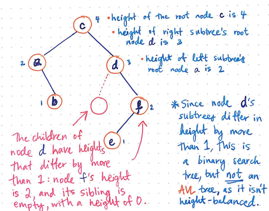
The height of the entire tree is 4, since the path from the root to the longest leaf e is 4 nodes. The height of the left subtree is 2, since the root node, a, of the left subtree has only one leaf, meaning that the longest path from a to b is 2 nodes. Similarly, the height of the right subtree is 3, since the longest path from the right subtree’s root d to e, is 3 nodes.
The children of node d have heights that differ by more than one level; node f’s height is 2, while its sibling, the left subtree of node d, is empty, with a height of 0. Since node d’s subtrees differ in height by more than one level, this is certainly not an AVL tree, as it violates one of the key rules of an AVL.
Okay, so this is not an AVL tree; but, we know that an AVL tree would be super useful, right? So, how can we turn this tree into an AVL tree?
Well, since we know the rules for an AVL tree, and we know how to make it a height-balanced tree, we could potentially try to rearrange these nodes in such a way that this currently unbalanced tree will quickly become height-balanced.
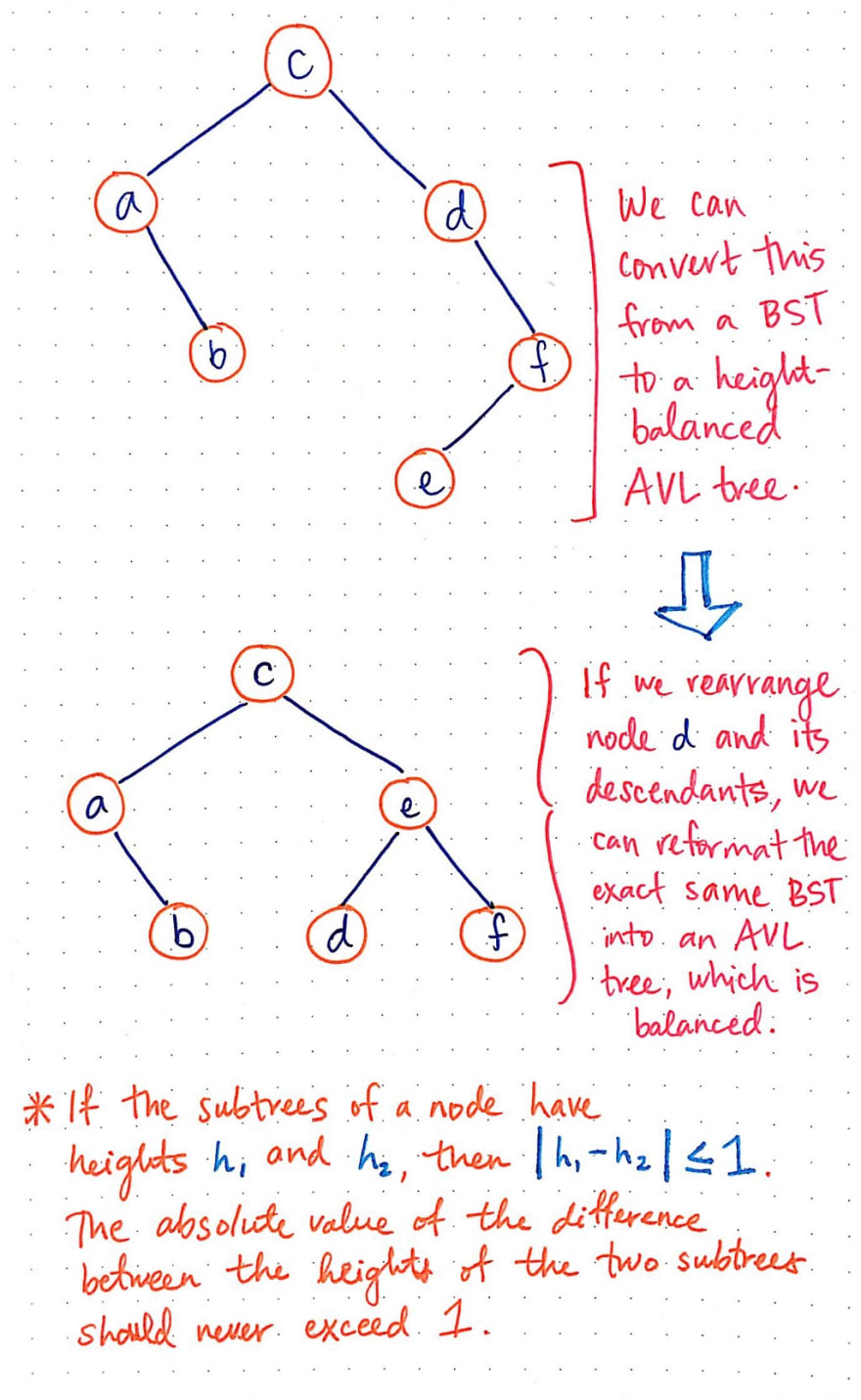
If we rearrange node d and its descendants, we can reformat the exact same BST we were just dealing with into an AVL tree, which is balanced. All we’ve done, really, is shifted around the right subtree. Where the right subtree once had a root node of d, it now has a root node of e, with two children beneath it.
The logic for how we rearranged those nodes stems from the balancing formula that every AVL tree will adhere to: if the subtrees of a node has heights h1 and h2, then the absolute value of the difference of those two heights must be less than or equal to (≤) 1. In other words, the difference between the heights of two subtrees in an AVL tree should never exceed 1 level.

The idea of “never exceeding 1 level” of height difference between two subtrees is also known as the balance factor. The balance factor is the difference in heights of its two subtrees. In a height-balanced tree, the balance factor can either be 0, -1, or 1, hence the reasoning for taking the absolute value between to subtrees and checking that the absolute value in their difference is under 1. The balance factor is how an AVL tree determines whether or not any given subtree of a tree is balanced or not.
So what happens if an AVL tree figures out that a tree isn’t balanced? Sure, we know that we can turn an unbalanced tree into a proper, height-balanced one. But how do we even go about doing this if (and when) we need to?
Time to find out!
Clever modifications for clever trees
We can think of AVL trees as a super clever set of scales, which can just magically balance themselves out evenly, no matter what you put on them. And, what’s more, no matter what you choose to be the center point of the data, the AVL “scales” will reconfigure itself so that the data is reorganized to be as balanced as possible.
For example, in the unbalanced BST we initially looked at, our input data was ordered and inserted in a descending manner, which made our AVL “scales” look very lopsided. In order to self-balance this tree the way that an AVL tree would do, we’d need this tree to be even on both sides of the “scales”, so that no matter what the root node is, the scales and subtrees would balance out correctly.

Except, of course, that AVL trees aren’t doing this work of balancing themselves magically. Rather, they’re employing a lot of logic under the hood, which perhaps makes them seem magical (and a tad bit intimidating, I’ll admit)!
So what exactly is this logic? Well, to be totally honest, it really is nothing more than some fancy node swapping! If you’re feeling like you’ve heard of this before, it’s because you have. We dealt with node swapping back when we were learning about heaps; in order to maintain the structure of a heap, we had to swap nodes in order to keep both the correct order of nodes as well as the correct heap structure.
In the context of height-balancing trees, the correct term for this kind of “glorified node swapping” is “rotations”. When it comes to AVL trees, there are two main types of rotations to use in order to rearrange nodes in a tree and do the hard work of self-balancing: single rotations and double rotations.
Single rotations are by far the simplest way to rebalance an unbalanced tree. There are two types of single rotations: a left rotation and a right rotation. A left rotation is useful if a node is inserted into the right subtree of another, higher up node’s right subtree, and that insertion or a deletion causes a tree to become unbalanced.
In the image shown here, a left rotation is performed on an unbalanced tree, with a root node of 1, and a right subtree with a node of 2, with its own right subtree/node of 3.
![]()
Since this tree is currently unbalanced, we swap the right subtree and perform a left rotation to make node 1 the left subtree of 2. This not only maintains the numerical order/structure of the elements as one would expect for a BST, but it also balances the tree so that both 1 and 3are in their correct locations relative to the new root node, 2.
As you might have already guessed, a right rotation is the exact opposite of this scenario. If a node is inserted into the left subtree of another child node’s left subtree (and the tree becomes unbalanced as a result), then we can perform a left rotation on the tree, so that 9, the former left subtree of the root node 10, becomes the new root node, and 8 and 10 become its respective left and right subtrees.
Sometimes, however, a single rotation just won’t cut it. In those scenarios, desperate times call for double rotations: namely, either a left-right rotation, or a right-left rotation. And yes, they probably are implemented in exactly the way that you expect they would be.
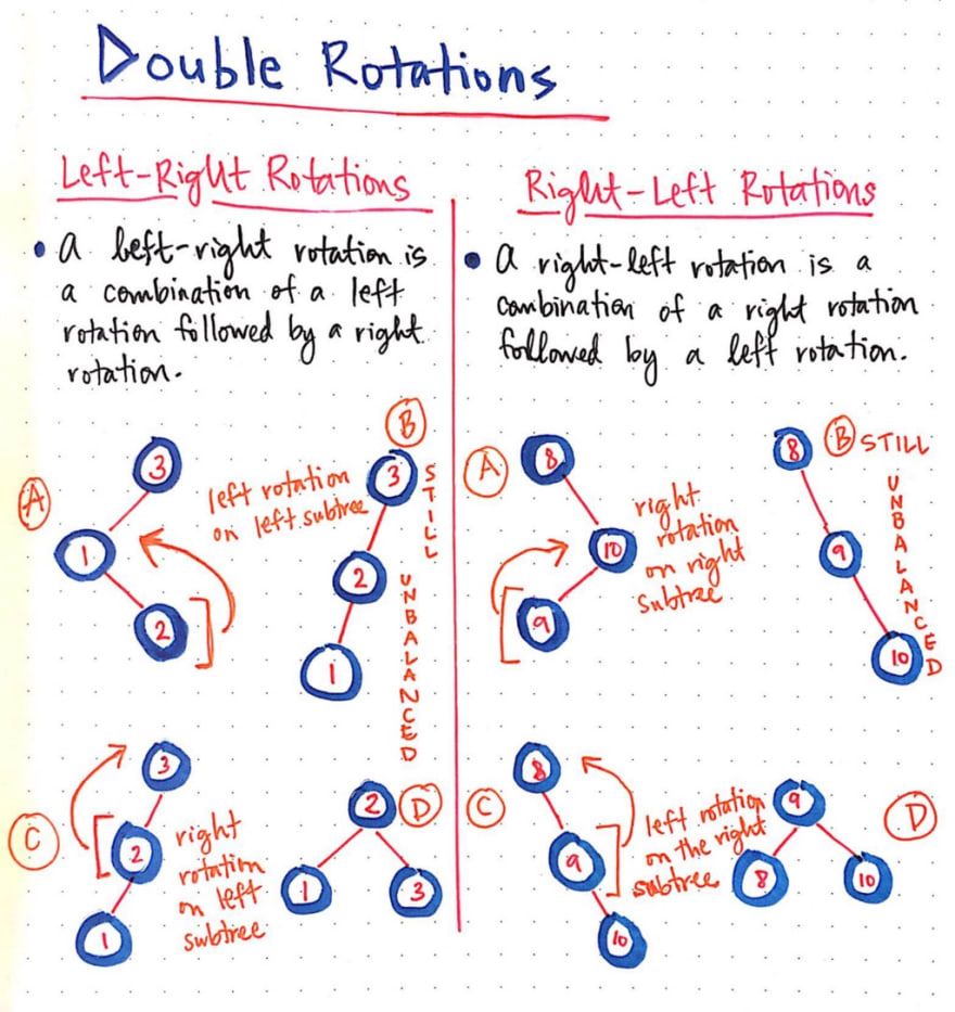
A left-right rotation is a combination of a left rotation, followed by a right rotation. In the examples shown here, we perform a left-right double rotation on the tree with a root node 3, a left subtree with a node 1, with its own right subtree and a node of 2. Once we perform a left rotation on the left subtree, our tree is a little easier to deal with. Our tree has transformed from 3–1–2 into 3–2–1. We’re back to something familiar: a left subtree of a left subtree. Since we already know how to handle those kinds of trees, we can easily perform a right rotation on the left subtree, so that 2 is now the new root nodes, and 1 and 3 are its children.
Conversely, a right-left rotation is the exact same thing, but in the reverse order. A right-left rotation is a combination of a right rotation followed by a left rotation.
And thus, with some super fancy swapping, these clever trees do some very important and smart work: they make sure that we can leverage the awesomeness of binary search trees and their efficient runtime. AVL trees are amazingly helpful in ensuring that, no matter what we add or remove from an AVL tree, our structures are smart and flexible enough to rebalance themselves and handle whatever we throw their way! And for that, I am deeply grateful that someone else was around to ask these tough questions (and come up with an elegant solution) over half a century ago, before you or I even could.
Resources
There are a whole host of resources out there on AVL trees, if you just know what to Google for when you search for them. Height-balanced trees are a pretty common concept in core computer science classes, so they are usually covered in CS curriculum at some point or another. If you’re looking for some further reading (that isn’t too math-heavy just yet), the links below are a good place to start.
- AVL Trees, AVL Sort, MIT Department of Computer Science
- Data Structures and Algorithms – AVL Trees, Tutorialspoint
- AVL Trees, Professor Eric Alexander
- How to determine if a binary tree is height-balanced, Geeksforgeeks
- Balanced Binary Search Trees, Professor Karl R. Abrahamson
- Height-Balanced Binary Search Trees, Professor Robert Holte
This post was originally published on medium.com


Top comments (0)