Making Sense of Merge Sort [Part 2]

This is the second installment in a two-part series on Merge Sort. If you haven’t read Part 1 of this series, I recommend checking that out first!

Last week, in part 1 of this series, we discovered a new type of sorting algorithm that’s different from anything we’ve learned about so far. I’m talking, of course, about merge sort! Merge sort is unique from other sorting algorithms we’ve covered in a handful of ways.

For starters, merge sort is a divide and conquer algorithm, meaning that it sorts a set of data by dividing it in half, and applying the same sorting logic to small “subsections” or “subproblems” in order to sort the larger dataset. Secondly, we know that merge sort is a smarty-pants algorithm that uses recursion; in other words, it calls upon itself from within itself! We also learned that merge sort is distinct from other sorting algorithms like insertion sort, selection sort, and bubble sort, because it’s a whole lot faster in running time than any of these other three algorithms.

Well, okay, okay, hang on for a second–how do we even know this to be a fact? We’re not ones to just believe things because someone else told us that it’s true! Nope, nope nope, we have to understand this for ourselves, because otherwise, what’s the point? We have to figure out why merge sort is faster. And when we say that it’s faster…just how fast is it? How does merge sort compare to other algorithms, in other respects? And why should we care?

Time to find out!

Return of the logs

Before we get into answering all of these deep questions, let’s first remind ourselves what a merge sort algorithm is, exactly. In case you need a quick refresher, the short story is that a merge sort algorithm divides a collection into half, sorts each half recursively, and then merges them back together.

This algorithm has two important core concepts at play. The first is “divide and conquer”, which divides each of those two halves in the same way, splitting the sublists down into one element each, before starting on the work to merge them back together again. The second is recursion, which we can see more clearly in a code example. In our mergeSort function from last week (adapted from Rosetta Code’s JavaScript implementation of merge sort), we can see that the mergeSort function actually calls itself.

function mergeSort(array) {
  // Determine the size of the input array.
  var arraySize = array.length;

  // If the array being passed in has only one element
  // within it, it is considered to be a sorted array.
  if (arraySize === 1) { 
    return; 
  }

  // If array contains more than one element,
  // split it into two parts (left and right arrays).
  var midpoint = Math.floor(arraySize / 2);
  var leftArray = array.slice(0, midpoint);
  var rightArray = array.slice(midpoint);

  // Recursively call mergeSort() on
  // leftArray and rightArray sublists.
  mergeSort(leftArray);
  mergeSort(rightArray);

  // After the mergeSort functions above finish executing,
  // merge the sorted leftArray and rightArray together.
  merge(leftArray, rightArray, array);

  // Return the fully sorted array.
  return array;
}

function merge(leftArray, rightArray, array) {
  var index = 0;

  while (leftArray.length && rightArray.length) {
    console.log('array is: ', array);
    if (rightArray[0] < leftArray[0]) {
      array[index++] = rightArray.shift();
    } else {
      array[index++] = leftArray.shift();
    }
  }

  while (leftArray.length) {
    console.log('left array is: ', leftArray);
    array[index++] = leftArray.shift();
  }

  while (rightArray.length) {
    console.log('right array is: ', rightArray);
    array[index++] = rightArray.shift();
  }

  console.log('** end of merge function ** array is: ', array);
}

What happens when we run this code? Well, let’s try sorting an array of of eight elements: [5, 1, 7, 3, 2, 8, 6, 4]. I’ve added some console.log's to make it a little bit easier to see how this algorithm works under the hood.

var array = [5, 1, 7, 3, 2, 8, 6, 4];

mergeSort(array);

> array is:  (2) [5, 1]
> left array is:  [5]
> ** end of merge function ** array is:  (2) [1, 5]
> array is:  (2) [7, 3]
> left array is:  [7]
> ** end of merge function ** array is:  (2) [3, 7]
> array is:  (4) [5, 1, 7, 3]
> array is:  (4) [1, 1, 7, 3]
> array is:  (4) [1, 3, 7, 3]
> right array is:  [7]
> ** end of merge function ** array is:  (4) [1, 3, 5, 7]
> array is:  (2) [2, 8]
> right array is:  [8]
> ** end of merge function ** array is:  (2) [2, 8]
> array is:  (2) [6, 4]
> left array is:  [6]
> ** end of merge function ** array is:  (2) [4, 6]
> array is:  (4) [2, 8, 6, 4]
> array is:  (4) [2, 8, 6, 4]
> array is:  (4) [2, 4, 6, 4]
> left array is:  [8]
> ** end of merge function ** array is:  (4) [2, 4, 6, 8]
> array is:  (8) [5, 1, 7, 3, 2, 8, 6, 4]
> array is:  (8) [1, 1, 7, 3, 2, 8, 6, 4]
> array is:  (8) [1, 2, 7, 3, 2, 8, 6, 4]
> array is:  (8) [1, 2, 3, 3, 2, 8, 6, 4]
> array is:  (8) [1, 2, 3, 4, 2, 8, 6, 4]
> array is:  (8) [1, 2, 3, 4, 5, 8, 6, 4]
> array is:  (8) [1, 2, 3, 4, 5, 6, 6, 4]
> right array is:  [8]
> ** end of merge function ** array is:  (8) [1, 2, 3, 4, 5, 6, 7, 8]
>> (8) [1, 2, 3, 4, 5, 6, 7, 8]> 

Rad! Look at all of that merging going on! Because of all the things that we’re logging out, we can see how this algorithm recursively just keeps on dividing elements until it has single-item lists: for example, it starts off with [5] and [1]. We can also see that, as we merge together two sublists and build up our array, we’re also doing the work of sorting the elements and putting them in their correct order. Notice how this happens with the two sublists of [1, 5] and [7, 3]. This algorithm uses a temporary structure (usually an array), and adds the sublists to that temporary array, in sorted order. Only after the sublists have been sorted and added will it actually proceed to copy those “sorted sublists” into the original array.

But back to our original mission: merge sort’s speed and efficiency. In order for us to understand that, we need to look at how must time it takes for the merge sort algorithm to do the work of 1) dividing the collection, 2) sorting it, and 3) merging it all back together.

Well, neither dividing the collection nor sorting it is the worst part of this algorithm. Because we’re using recursion – and because we’re splitting each half into halves recursively – the work of dividing the collection isn’t too expensive. Furthermore, since we sort two items at a time using a comparison operator (like < or >), we know that this, too can’t be all that expensive – it should take a constant amount of time.

Instead, the most expensive part of any merge sort algorithm is the work of merging, itself – the work of putting back together the small sublists, in sorted format. If we go back and look at our code again, we can see that the work of merging is actually taking up the most amount of time, and what is logged out the most often, too.

Thus, we’ll focus on the aspect of merging, since that’s what is responsible for giving the algorithm it’s time complexity. So, what do we mean when we say ‘merging’?

When we use the term ‘merging’, what we’re actually referring to is the act of appending an item – in sorted order – to the temporary array structure, which we build up over time as we continue to sort and append more items to it.

After the merge sort algorithm has recursively divide up the unsorted list into single-item elements, we can say that, since each list has only one item in it, everything is sorted (but obviously not joined together yet). The step of merging involves comparing two sublists, and then appending the larger one to the end of the smaller one.

This will probably make a bit more sense with an example:

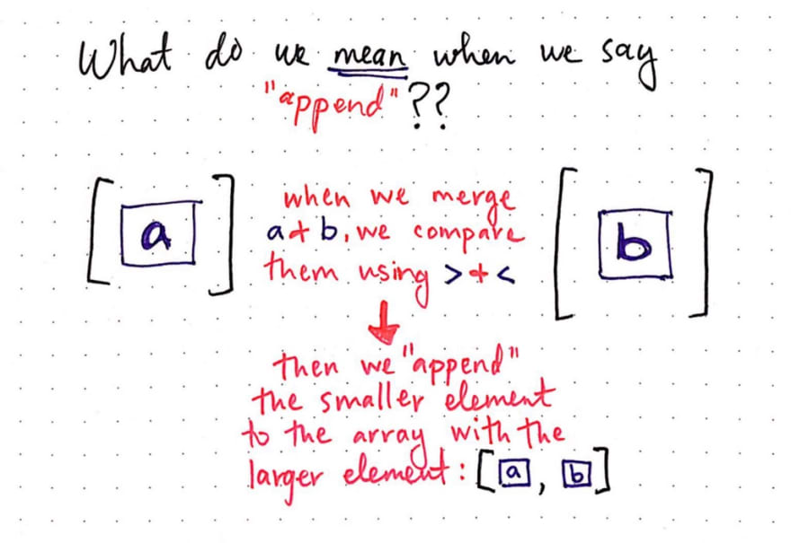
In the example above, we can imagine that we’re sorting a large dataset, and we’re at the point now where we’ve divided the collection down to its recursive base case: the point where each list has only one element in it. Here, we have two sublists, one with the element a and another with the element b. In order to merge these two items together, we must determine which of the two is smaller (using a comparison operator), and then append one element to the other.

If we look at different merge sort algorithm implementations, we’ll probably notice pretty quickly that people will often write their merge functions in slightly different ways, depending on whether they’re using the greater than (>) or less than (<) operator. Regardless of individual implementations, however, the basic idea of how we do the work of merging tends to remain the same.

Okay – in this particular example, we had two lists, each with only one element in it. We had to perform a single append operation in order to merge them together. Realistically however, we’re never really going to be sorting a list of two items, right? Instead, we’ll be dealing with a much larger dataset. Let’s see how many times we’d have to append elements with a bigger unsorted collection. In the example shown below, instead of two items, we have a collection of eight items that need to be sorted.

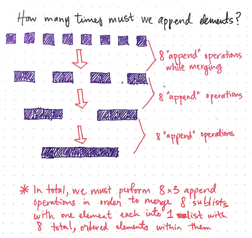
We’ve already done the work of dividing, and now we’re ready to start merging things together. We begin with eight, individual items in eight lists – remember that they’re considered “sorted” because there’s only one item in them! We want to combine them together such that we have half as many lists. If we think about it, this makes sense: when we were dividing, we were doubling the number of lists until we reached our base case of one item per list. Now, we’re doing the exact opposite in order to build our list up.

To start, if we have eight items, we need to merge them together in sorted order such that we have just four items. This means we’ll need to perform eight “append” operations.

Remember that an “append” operation involves two steps:

1. comparing the items that we want to combine together, and
2. inserting them into our temporary array in sorted order

Effectively, we’ll need to perform one append operation per item. Once we’ve done that, we’ll end up with four lists, with each list’s elements in sorted order. Great!

Next step: we’ll need to merge our four lists together so that we have just two lists. We’ll again need to perform eight append operations in the process of comparing, sorting, and inserting the elements into their correct places.

Alright, now we’re down to just two lists, with four sorted elements in each of them! You know what’s coming, right? We’ll perform eight append operations, and end up with one single, sorted list that has eight elements within it.

Great! We’re done sorting – finally! Let’s take a step back and look at what just happened. In total, we performed (8 + 8 + 8), or 24 append operations in order to turn out single-element sublists into one, sorted list. In other words, we performed 8 × 3 append operations. I’m repeating this a few different times, because there’s a special relationship between those numbers, which you might remember from an earlier post.

If not, don’t worry! We’ll look at some more examples and see if we can identify the relationship and any patterns.

Logarithms strike back – but like, in a nice way

One of my favorite authors once wrote that “Brevity is the soul of wit”, and I tend to believe him. So, rather than illustrate a ton of long examples, I’ve just listed out how many append operations they’ll require.

We already know that, when the number of elements in the list, which we’ll call n, is 8, our merge sort algorithm will perform 8 × 3 append operations.

When n = 16, we must perform 16 × 4 append operations. When n = 4, merge sort will perform 4 × 2 append operations. And when n = 2, merge sort will perform 2 × 1 append operations.

If we abstract out n in each of these scenarios, we’ll start to see something familiar emerge.

Tada! Logarithms are back. If you’re unfamiliar with how logs work, check out this post from earlier in the year. I promise that it’ll give tons more context on what’s happening here.

If we abstract out n, we’ll see that in all of these examples, one truth seems to be evident:

If we multiply the log of n by the value of n, the result ends up being the number of total append operations to perform.

So what does that mean, exactly? I think that this statement can be a little bit confusing, but it should (hopefully) make more sense if we visualize it. Let’s return to our original example of performing merge sort on a list of eight elements:

Here, we can see more clearly how exactly we are multiplying n, the total number of items, by the log of n. You might see this written in a few different ways, such as (n â‹… log n), (n × log n), or just (n log n). Don’t be tripped up by them – they’re all equivalent. All of these notations are pronounced “n log n”, and they’re a fairly common in the context of sorting algorithms!

Now that we know it takes (n × log n) append operations to do the work of merging in a merge sort algorithm, we probably have one question: what does this even mean? As in – is this a good thing? Is it fast? Or slow? Or…somewhere in between?

Well, now that we’ve abstracted out the amount of time it takes to merge together n number of elements, we can just try out different values for n, and see how merge sort changes as n grows in size! Let’s try out some larger datasets, and see how many operations merge sort would take in order to sort them.

In the example show here, we can see that as n grows, the number of operations also grows. However, it’s not quite as terrible as when we were working with bubble sort, insertion sort, or selection sort; in each of those algorithms, as n doubled in size, the amount of time it took to perform the algorithm would quadruple, giving each of these algorithms a quadratic runtime.

But what’s going here? The number of operations isn’t growing quadratically…but it’s also not growing linearly, either. Well, as it turns out, we’ve stumbled upon something new entirely. And, if we think about it a little more deeply, it might start to become obvious.

Given the fact that the amount of time that merge sort needs to run is (n × log n), there’s clearly both a linear and a logarithmic aspect at play here.

The combination of linear and logarithmic time is referred to as linearithmic time, and that’s exactly what the merge sort algorithm’s time complexity happens to be!

You might sometimes see (n log n) referred to as “quasilinear” or “loglinear” time, but both of these terms are also used in the context of economics or mathematics. I tend to prefer the term “linearithmic” because it’s always used in the context of Big O time complexity of an algorithm.

So, how does a linearithmic runtime compare to other time complexities that we’ve seen so far?

Well, obviously it’s not as ideal something that has a constant runtime, or O(1). It’s also not nearly as fast as a binary search algorithm – despite the fact that merge sort uses a similar divide and conquer strategy – which runs in logarithmic, or O(log n), runtime. It’s also slightly worse than an algorithm that runs in linear time (O(n)). However, we can see how it performs so much better than an algorithm that has a quadratic runtime (O(n²)). In fact, that’s what makes merge sort so different from the sorting algorithms we’ve looked at so far! Generally speaking, it’s hard to find a sorting algorithm that performs faster than linearithmic time; as we’ve discovered from our adventures, the majority of them run in quadratic time.

The (merge sort) force awakens

We’ve completely exhausted the time complexity of merge sort ( linearithmic ), and how it compares to other sorting algorithms. But of course, time complexity isn’t everything. As we’ve learned, there are plenty of other considerations when it comes to picking a sorting algorithm.

It’s time to take a look at how merge sort stacks up compared to its siblings!

Earlier, when we were running our code, we learned that a standard merge sort algorithm requires a temporary array structure in order to sort and append elements. In other words, it requires a constant, or O(n), amount of space – the memory needed for the temporary buffer array. Merge sort needs O(n) amount of memory in order to copy over elements as it sorts. This is probably the greatest drawback of the merge sort algorithm: it is an out-of-place sorting algorithm, that requires additional memory as its dataset grows.

However, merge sort has some helpful aspects, too. Because it compares two elements at a time, using a comparison operator, if two elements are equal, it won’t change their order as it merges them together. Thus, merge sort maintains the stability of its inputted dataset, and can be classified as a stable sorting algorithm. And, since it uses a comparison operator to compare two elements, it’s also a comparison sort. We’ve also become pretty familiar with the concept of recursion in the context of merge sort, which we know that the algorithm relies heavily upon; thus, merge sort is a recursive algorithm.

Perhaps the most useful thing about merge sort – aside from the fact that it’s substantially faster when compared to other sorting algorithms – is how good it is at sorting large datasets. Because merge sort is often implemented as an external sorting algorithm, it can do the work of sorting outside of main memory, and then later can pull the sorted data back into the internal, main memory.

In fact, there’s a chance that you are dealing with merge sort all the time as a developer or consumer of a programming language. For example, Ruby’s Array::Enumerable class has a sort,sort!, and sort_by method. If you take a look at the source code for these methods, you’ll see that they all lean on a method called sort_inplace, which – you guessed it – implements merge sort under the hood.

What’s even cooler is that if we take a look at the comment left behind in the code, we can find the explanation of this method is intended to work:

Sorts this Array in-place.> The threshold for choosing between Insertion sort and Mergesort is 13, as determined by a bit of quick tests.

How cool is that!? Ruby’s own Array#sort method was implemented intelligently enough that it knows to use insertion sort for smaller arrays, and merge sort for larger ones. As it turns out, this is pretty commonplace in other programming languages, too. Both Java and Python, for example, implement Timsort, which is a hybrid of insertion sort and merge sort, under the hood of their sorting methods.

Who knew that merge sort was all around us this entire time!? Well, now we both know – and we’re all the powerful for it.

Resources

Still can’t get enough merge sort? Want to learn more about logarithms? Or do you just want to merge sort all of the things? These resources are a good place to start learning more.

1. Data Structures – Merge Sort Algorithm, TutorialsPoint
2. Linearithmic Complexity, Kevin Drumm
3. Divide and Conquer: Merge Sort, Professor Michelle Hugue
4. Logarithm Calculator, 1728 Software Systems
5. Analysis of Merge sort algorithm, mycodeschool

This post was originally published on medium.com