updated 2020-01-24
-noted that the example in part 2 will use S2, not Geohash
-removed "relational" term when discussing spatial data types
Google Maps, Yelp, and Meetup all can help us answer a variation on the same question of "what X is nearest to Y". What subway stop is closest to my friend's house, where's the nearest sushi place, who else is interested in hiking in my town, etc. These sites use geographic data about points of interest, and our current location or a location of our choosing to calculate what's close.
In this post, I'll discuss how we can make these types of calculations in our own apps. Because of the number of points in these datasets and the number of visitors querying the datasets, we will be looking at not only how to make these calculations, but also how to make them faster and more efficient.
We'll start by looking at points of interest on a line, then move our way up to 2d planes and then a globe. Along the way we'll encounter geohashing, an elegant solution to the problem of nearness.
Staying Close in Lineland
Let's imagine a world with one-dimension. All points are described by a single value, the relative position on that single great line of existence. To avoid any unfortunate incidents, we can stay in our 3d world and just observe this lineland from afar.

We see 5 points of interest on the line, with the following positions:
Place of Interest: Position on Line
"The Red Fox Tavern": -5
"Charlie's Chicken Shack": -3
"Smoothie Town": 0
"The Wilted Cauliflower": 2
"Eggplant Paradise": 4
With only one-dimension, the distance between any two points in lineland is simply the difference in their positions. If we want a lineland Yelp clone to answer the question of what restaurants are within 5 units of my house at position 1, we can use a brute-force approach by calculating the distance from every point to the center point:
Distances from Points of Interest to 1
"The Red Fox Tavern": -5 => 1 - (-5) => 6
"Charlie's Chicken Shack": -3 => 1 - (-3) => 4
"Smoothie Town": 0 => 1 - 0 => 1
"The Wilted Cauliflower": 2 => 1 - 2 => -1
"Eggplant Paradise": 4 => 1 - 4 => -3
We find three restaurants in the specified range.
As our dataset of points of interest grows larger, calculating the distance from every point to the center point is more and more work and our algorithm gets slower (or we parallelize the calculation and spend more computation in exchange for time).
To keep the size of dataset manageable in our example, we can modify our algorithm to return all restaurants in the position range of -4 through 6, taking the farthest allowable distance to the left through the farthest allowable distance to the right.

Despite it's range of culinary delights, there's not much going on in lineland, so let's bump up another dimension.
Infinite Planes and the Distance Formula
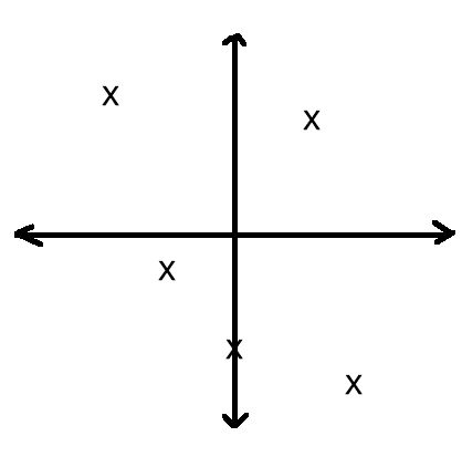
We are now in the world of two-dimensions, with the familiar X and Y coordinate system of geometry and mathematics. We plot points of interest on an infinite plane, with a horizontal X position and vertical Y position.
In our plane world, we see the same 5 restaurants from lineland, but with positions composed of X and Y pairs:
Place of Interest: (X, Y) coordinates
"The Red Fox Tavern": (-5,8)
"Charlie's Chicken Shack": (-3,-1)
"Smoothie Town": (0,-4)
"The Wilted Cauliflower": (2,7)
"Eggplant Paradise": (4,-6)
With two-dimensions the distance between any two points is calculated using a derivation of the Pythagorean theorem, the Distance formula, the square root of the squares of the differences:
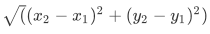
In our 2d Yelp clone, we want to find restaurants within 5 units of my house at position (1,2). Again, we start with brute-force and do the calculation for every point to the center point:
Distances to (1,2)
"The Red Fox Tavern": (-5,8) => sqrt((-5 - 1)*(-5 - 1) + (8 - 2)*(8 - 2)) => 7.75
"Charlie's Chicken Shack": (-3,-1) => sqrt(16+9) => 5
"Smoothie Town": (0,-4) => sqrt(1+36) => 6.08
"The Wilted Cauliflower": (2,7) => sqrt(1+25) => 5.10
"Eggplant Paradise": (4,-6) => sqrt(9+64) => 8.54
Doing this calculation for 5 points is no big deal, but as the dataset grows larger, our algorithm needs more and more compute capacity and/or time. As with lineland, we address scalability by limiting the size of the dataset. The fewer points to feed into the distance formula, the faster.
To limit the size of the dataset we use a minimum bonding rectangle or bounding box:
The minimum bounding rectangle (MBR), also known as bounding box (BBOX) or envelope, is an expression of the maximum extents of a 2-dimensional object (e.g. point, line, polygon) or set of objects within its (or their) 2-D (x, y) coordinate system, in other words min(x), max(x), min(y), max(y). The MBR is a 2-dimensional case of the minimum bounding box.
As the diagram below illustrates, we can create a bounding box that is guaranteed to include at least all the points within R units of the center point. Given a point at (x, y), the four corners of the box will be at:
Upper Right Corner: ((x + r), (y + r))
Lower Right Corner: ((x + r), (y - r))
Lower Left Corner: ((x - r), (y - r))
Upper Left Corner: ((x - r), (y + r))

With these outer bounds defined, we can restrict the set of points we calculate the distance for to be only points between these bounds.
In pseudocode, our approach becomes something like:
- Pick a center point and how far out we are going to look (the distance)
- Calculate a bounding box around the center point, based on the distance
- Find the subset of the points of interest with a X between the min and max X of our bounding box and Y between the min and max Y of our bounding box
- For each point in the bounding box, run the Distance formula to calculate distance from the center point
- Return points whose distance to the center point is within the desired distance
Without getting into the technical details here, most data stores have indices that support range queries to make finding the subset of points within the bounding box efficient.
With that, we're ready to enter the third dimension and think about distances over a spherical object, like say planet Earth.
Spheres, Latitude, Longitude and the Haversine Formula
While we use street addresses to locate places in our everyday lives, under the covers we are all using latitude and longitude coordinates:
The combination of these two components specifies the position of any location on the surface of Earth, without consideration of altitude or depth.
From GISGeography's site: Latitude coordinates are essentially Y-values between -90 and 90 degrees with 0 at the Equator. Longitude values are essentially X-values between -180 and 180 degrees with 0 at the Prime Meridian.
For example, the latitude and longitude of the Washington Monument is 38.8895°, -77.0353°.
Before we move on, it is important to note that calculating the exact distance between points on Earth is far more complex than for points on a two-dimensional plane. Fortunately, for the scenarios we are concerned with, say locating the nearest taco stand, we are OK with simplifying our distance calculations at the expense of precision by making these assumptions:
- The Earth is a perfect sphere (it's actually an oblate spheroid)
- All points of interest are directly on the surface of the Earth, i.e. we ignore elevation changes
With these assumptions in place, let's take a look at the 5 points of interest from our prior examples, now specified by latitude and longitude coordinates:
Place of Interest: (Latitude, Longitude) coordinates
"The Red Fox Tavern": 32.7549°, -117.1425°
"Charlie's Chicken Shack": 32.7524°, -117.1427°
"Smoothie Town": 32.7376°, -117.1714°
"The Wilted Cauliflower": 32.5229°, -117.1165°
"Eggplant Paradise": 32.5073°, -117.0855°
Me drawing those points on a sphere isn't going to help anyone, but if you are curious, these are all just locations selected around San Diego and Tijuana.
To calculate the distance between points on Earth with latitude and longitude, many software packages use the Haversine formula, a type of great-circle distance calculation. The idea of great-circle distance is:
the shortest distance between two points on the surface of a sphere, measured along the surface of the sphere (as opposed to a straight line through the sphere's interior). The distance between two points in Euclidean space is the length of a straight line between them, but on the sphere there are no straight lines. In spaces with curvature, straight lines are replaced by geodesics. Geodesics on the sphere are circles on the sphere whose centers coincide with the center of the sphere, and are called great circles
The Haversine formula itself is described in great detail on the Wikipedia page if you want to flex your geometry muscles. Lots of sines and cosines. The phi variables are latitude, the lambda variables are longitude:

In our 3d Yelp clone, we want to find restaurants within 5 miles of my house at 32.7584°, -117.1402° (not actually my house). Again, we start with brute-force and do the calculation for every point to the center point (in this case using an online calculator to avoid doing the math myself):
Distances to 32.7584°, -117.1402°
"The Red Fox Tavern": 32.7549°, -117.1425° => 0.276 miles
"Charlie's Chicken Shack": 32.7524°, -117.1427° => 0.44 miles
"Smoothie Town": 32.7376°, -117.1714° => 2.315 miles
"The Wilted Cauliflower": 32.5229°, -117.1165° => 16.339 miles
"Eggplant Paradise": 32.5073°, -117.0855° => 17.649 miles
Many modern data stores have support for storing latitude and longitude pairs, as well as built-in functions for calculating the distance between these points. Typically these features or packages are called Spatial Data support or GIS (Geographic information system) support.
Even it is built-in to the data store, this type of calculation can get more and more expensive as we increase the size of our dataset. Again, our approach to limit computational and time use is to limit the dataset we operate on.
Conceptually, like with planes, we want to only calculate the distance between points that are within a bounding box around the center point. One method for calculating the edges of such a bounding box using latitude and longitude is described in this paper. The linked paper suggests that this method could be used with a SQL-compliant datastore to leverage latitude and longitude indices to select the subset of points in the bounding box and only then calculate the distance. A similar approach using MySQL specifically, is detailed in this post. There are many more similar techniques I came across while writing this post. I haven't tested them to give a concrete recommendation of one over the other.
The solution I want to talk about is called geohashing.
Geohashing
Geohash is a public domain geocode system invented in 2008 by Gustavo Niemeyer[1] and (similar work in 1966) G.M. Morton[2], which encodes a geographic location into a short string of letters and digits. It is a hierarchical spatial data structure which subdivides space into buckets of grid shape, which is one of the many applications of what is known as a Z-order curve, and generally space-filling curves.
from https://en.wikipedia.org/wiki/Geohash

In other words, through geohashing you divide the world into a grid of squares and rectangles, addressed by hash. Any point on the earth (latitude and longitude) has a corresponding hash that fits into one of these grid cells or bins. To see a visual explanation of geohashing, check out this video or this page.
The length of the geohash we use determines how large the bin is. For example, a geohash length of 5 will give us an approximately 5 km by 5 km bin.
Geohashes were originally used as part of a URL-shortening service, but across the industry are now used for spatial indexing and searches as well.
To return to our Yelp-like example scenario of finding nearby restaurants, let's add 5 character geohashes to our points of interest:
Place of Interest: (Latitude, Longitude) coordinates | Geohash
"The Red Fox Tavern": 32.7549°, -117.1425° | 9mudq
"Charlie's Chicken Shack": 32.7524°, -117.1427° | 9mudq
"Smoothie Town": 32.7376°, -117.1714° | 9mudj
"The Wilted Cauliflower": 32.5229°, -117.1165° | 9mu9n
"Eggplant Paradise": 32.5073°, -117.0855° | 9mu8z
Again, my fake house is at my house at 32.7584°, -117.1402° or 9mudq.
A naive algorithm to find nearby points of interest would be to return points with the same geohash as the center point. This gets us some of the nearby points of interest, but depending on the distance we want to search, likely leaves out nearby points of interest that are in neighboring geohash bins.
To get a more comprehensive set of points of interest, we can get all the points in the center geohash bin and its 8 immediate neighbors. From there, assuming we want to be precise, we calculate the distance between all the points and the center, dropping the points that are too far away.
Like a bounding box algorithm, a geohash based algorithm can handle larger datasets by first chopping those datasets into manageable chunks for our distance calculations. Also, while the latitude and longitude based bounding boxes described above depend on the data store having support for spatial data, we can manipulate geohashes in any data store, as they are just strings.
The ability to use geohashes without custom spatial data types will come in handy in my next post, where I dig into a solution I studied that uses DynamoDB as a data store, along with some JavaScript functions to implement a simple Starbucks locator. This solution actually uses Google's S2 as a different type of geohash, which I'll explain. In that post, I'll also get into two issues of some importance that I glided past here: first, deciding how big a geohash to use in your application and second, how to find the neighboring geohash bins.
See you then!


Top comments (0)