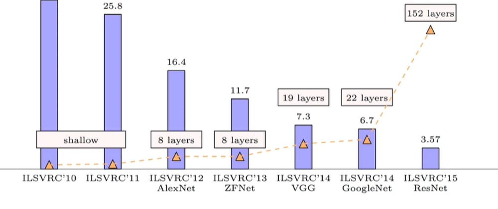

1.ILSVRC’10
2.ILSVRC’11
3.ILSVRC’12 (AlexNet)
4.ILSVRC’13 (ZFNet)
5.ILSVRC’14 (VGGNet)
6.ILSVRC’14 (GoogleNet)
7.ILSVRC’15 (ResNet)
- ILSVRC stands for Imagenet Large Scale Visual Recognition Challenge or the Imagenet Challenge .
- ILSVRC is a challenge which is held annually to allow contenders to classify the images correctly and generate the best possible predictions .
AlexNet

- AlexNet CNN architecture won the 2012 ImageNet ILSVRC challenge by a large margin : it achieve a top-five error rate of 17% while the second best achieved only 26%
- It was developed by Alex Krizhevsky , Ilya Sutskever and Geoffrey Hinton .
- It is quite similar to LeNet-5, only much larger and deeper, and it was the first to stack convolutional layers directly on top of each other, instead of stacking a pooling layer on top of each convolutional layer.
- It consist of 8 convolutiona land fully connected layers and 3 max pooling layers .

To reduce overfitting, the authors used two regularization techniques: first they applied dropout with a 50% dropout rate during training to the outputs of layers F8 and F9. Second, they performed data augmentation by randomly shifting the training images by various offsets, flipping them horizontally, and changing the lighting conditions.
ZFNet

- ZFNet is another 8-layer CNN architecture .
- ZFNet is largely similar to AlexNet, with the exception of a few of the layers .
- ZFNet CNN architecture won the 2013 ImageNet ILSVRC challenge.
- One major difference in the approaches was that ZF Net used 7x7 sized filters whereas AlexNet used 11x11 filters.
- The intuition behind this is that by using bigger filters we were losing a lot of pixel information, which we can retain by having smaller filter sizes in the earlier convolution layers.
- The number of filters increase as we go deeper. This network also used ReLUs for their activation and trained using batch stochastic gradient descent.
VGGNet

- The runner up in the ILSVRC 2014 challenge was VGGNet .
- It was developed by K. Simon‐yan and A. Zisserman.
- During the design of the VGGNet, it was found that alternating convolution & pooling layers were not required. So VGGnet uses multiple of Convolutional layers in sequence with pooling layers in between.
- It had a very simple and classical architecture, with 2 or 3 convolutional layers, a pooling layer, then again 2 or 3 convolutional layers, a pooling layer, and so on (with a total of just 16 convolutional layers), plus a final dense net‐work with 2 hidden layers and the output layer. It used only 3 × 3 filters, but many filters.
GoogLeNet

- The GoogLeNet architecture was developed by Christian Szegedy et al. from Google Research,12 and it won the ILSVRC 2014 challenge by pushing the top-5 error rate below 7%.
- This great performance came in large part from the fact that the network was much deeper than previous CNNs
- This was made possible by sub-networks called inception modules, which allow GoogLeNet to use parameters much more efficiently than previous architectures: GoogLeNet actually has 10 times fewer parameters than AlexNet (roughly 6 million instead of 60 million).

*GoogLeNet uses 9 inception module and it eliminates all fully connected layers using average pooling to go from 7x7x1024 to 1x1x1024. This saves a lot of parameters .
Several variants of the GoogLeNet architecture were later proposed by Google researchers, including Inception-v3 and Inception-v4, using slightly different inception modules, and reaching even better performance.*
ResNet

- The ILSVRC 2015 challenge was won using a Residual Network (or ResNet)
- It was Developed by Kaiming He et al .
- It delivered an astounding top-5 error rate under 3.6%, using an extremely deep CNN composed of 152 layers. It confirmed the general trend: models are getting deeper and deeper, with fewer and fewer parameters. The key to being able to train such a deep network is to use skip connections (also called shortcut connections): the signal feeding into a layer is also added to the output of a layer located a bit higher up the stack. Let’s see why this is useful.

When training a neural network, the goal is to make it model a target function h(x). If you add the input x to the output of the network (i.e., you add a skip connection),then the network will be forced to model f(x) = h(x)-x rather than h(x). This is called residual learning .
References :
- https://www.guvi.in/ (Online Learning Platform)
- Handson Machine Learning with Scikit (Reference Book , PDF - https://drive.google.com/file/d/16DdwF4KIGi47ky7Q_B- 4aApvMYW2evJZ/view?usp=sharing) .


Top comments (0)