
Hi All,
With my first contribution to the community I would like to share with you my knowledge about deep learning and its applications. This will consist of a series of posts which I call Deep Learning for Dummies, coming out approximately one post a month.
As of this special occasion, this is my first post, I would like to start thanking the Santander Dev community peers for their warm welcome and for giving me the opportunity to grow my knowledge collaborating at this amazing initiative.
I thought this series as both, a theoretical and practical introduction to Artificial Intelligence for someone who doesn't know anything about it. Expect to find easy-going language and explanations of all the concepts involved.
Below you have the lists of posts that I plan to publish under this series. I will keep it updated with each published post. Unpublished posts titles and used libraries can change:
- Introduction to Deep Learning, basic ANN principles
- Artificial Neural Networks: types, uses, and how they work
- CNN Text Classification using Tensorflow (February - March)
- RNN Stock Price Prediction using (Tensorflow or PyTorch) (April - May)
- Who knows? I may extend it. Perhaps some SNN use case.
This is a long one but I think totally worth reading, specially if you are new to this world. In my opinion, it gives you a good base for understanding how any deep learning algorithm works. Let's see the contents.
Table Of Contents
- What is deep leanring?
- Artificial Neurons
- Activation Functions
- Artificial Neural Networks (ANN)
- Learning process of an ANN
- Review of the whole trainining/learning process
- Final Thoughts
What is deep Learning ?
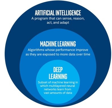
Figure one is a graphical representation of the concepts that I am going to describe below.
The term Artificial Intelligence was coined back in 1955 by John McCarthy in a workshop at Dartmouth College where attendees created algorithms to play checkers. John and its team invented the alpha-beta algorithm which is an improvement of the min-max algorithm. Those algorithms are designed to search the optimal move for the player, the one that minimize the loss and maximize the gain. Clicking on the examples, you can see that the unique part of those algorithms are their design. The developers developed the logic which the algorithm follows in order to calculate the best move. We will see that deep learning is completely different to this.
Machine Learning, a term coined by Arthur Samuel in 1959, is a subset of AI algorithms that use structured and labeled data to learn by themselves and make accurate predictions when a not labeled input is given. There are various machine learning algorithms, I will list some of the most popular in case you want to research and learn more about them: Naive Bayes, Random Forest, Support Vector Machine, K-Nearest Neighbor. The idea between this technique is that you create a model which, while learning or training, it modifies the mathematical function that describes its output till that function outputs an accurate prediction when and input is given. This is achieved by training and testing the model with previously labeled data.
See a visual example in the "figure 2". Let's say that we want to predict how many ice-creams are going to be sold based on temperature readings. We take the historic data of ice creams sold at different temperatures and plot it as a cluster of points in a 2-axis graph. Now our ML algorithm can be represented as a line which represents our prediction, meaning that if we want to know how many ice creams will be sold at 30º degrees, we just have to choose that point in the graph over the line and read the ice-creams axis, "y". The process of learning involves improving the shape of the line till it better represents the distribution of the points cluster. As you can realize, the importance of the data quality here is crucial, since a nonsense cluster of points will make it impossible for the algorithm to adjust the line properly.

This is similar to what deep learning does, the difference here is the method we use to do so. Deep Learning, term that was first introduced by Rina Dechter in 1986, is a subset of Machine Learning algorithms that focuses on performing the prediction task by mimicking the human brain structure. This is why it has associated terms such as artificial neurons and artificial neural networks, however, don't make the mistake to believe that our brain works in a similar way that deep learning algorithms do. Our biological nervous system is much more complex such that as of today we still don't completely understand how does our brain works. Artificial Neural Networks that we use in the deep learning algorithms are just an extremely simplified mathematical model of our brain strucutre.
Let's dig more into the deep learning components.
Artificial Neurons
As I stated above, Deep Learning is about designing algorithms that learn by themselves in a such a way that simulates our biological brain behavior. This is achieved thanks to the implementation of Artificial Neurons, and, when those are connected to each other they form what we know as an Artificial Neural Network.
In "figure 3" you can see the representation of an artificial neuron. It is nothing else than a series of mathematical functions where Xi are the inputs, Wi are the weights associated with every input, b is the bias unit and Y is the output. Ass we can see, the neuron computes the sum of the inputs multiplied by the weights, and then adds the bias term. After, it passes the result of this operation to the activation function. Finally, the output of the activation function "Y", is the final output of the neuron.

The value of the weights and the biases are assigned at the beginning when creating the algorithm, afterwards, those parameters are automatically updated through the training process. In fact, when a neural network is learning, it is updating the values of the weights and biases of each neuron till the output is the desired one. After training, those values can be stored and introduced to a copy of the neural network in another computer, which will perform with the same accuracy as the one we have been training. We will see more about this later on.
The role of the activation function is to encode the result of the summation between a fixed scale which has to be the same for all the neurons in the same layer, so the neural network can learn from the output of each neuron. When the algorithm is predicting, it bases its conlcusions on the relationships between the outputs of each neuron, this is the reason why we need the output of each neuron in the same layer to be scaled between the same range, so the algorithm can see what is the impact of every neuron from the same layer to the final output. This allows for correct weight and biases recalculation when training, what makes our model have a better prediction each time. We'll see what is a layer and how does the process of training works later on.
Activation Functions
The activation function is what we call the mathematical operation that the neuron performs over the sum of the inputs. One important aspect to consider is that neural networks used in industry consist of thousands of neurons and every single activation function has to be computed, then, the function has to be simple enough to reduce the computation complexity of the algorithm, allowing for quick predictions.
Now I am going to list the most popular activation functions employed in neural networks and you'll see they are extremely simple. Theoretically any given function can be used as an activation function, however, due to the reason covered in the paragraph above, those are the most common:
-
Sigmoid Function: This function represented in the figure 4 scales the output between 0 and 1, normalizing the output of each neuron. Its advantage is that the function is smooth, preventing unexpected jumps at the output. On the other hand, the main disadvantage is that scaling between 0 and 1 makes it difficult to differentiate clearly between a multiple set of large inputs, so we have a bad resolution. In addition, as we see on the graph, if the input is larger than 6 or smaller than -6, the output will allways be 1 or 0 respectively.

Figure 4 (Sigmoid activation function) -
Hyperbolic Tangent (TanH): This function represented in the figure 5 has a similar behavior as the softmax but scaling the output between -1 and 1 instead. The positive part is that we have a higher resolution, meaning that the we are able to differentiate better between similar inputs. It also allows the network to identify more features of the dataset, since the output can have both signs, plus and minus, so it helps the prediction. The negative part is that the slope of the function increased, decreasing the maximum input range that we can manage. If we have an input smaller than -3 or bigger than 3, the output will allways be -1 and 1 respectively.

Figure 5 (TanH activation function) -
Rectified Linear Unit (ReLU): This function represented in the figure 6 solves the problem of the big inputs. If the input is positive, it returns the same value, while if the input is negative is returns 0. The best part of this function is that it does not activates all the neurons at every input, reducing the computational complexity. On the other side, we don't have any sensibility for negative inputs. There are some modifications of this function that solves the problem of negative inputs insensibility, like the LeakyReLU. Another aspect to consider is that this function does not scale the output between a range, so depending on the problem you want to solve it may be the one you need or not.

Figure 6 (ReLU activation function) -
Softmax: This function represented in the figure 7 is different from the others and it is mainly used at the output layer when the task of the neural network is to classify the input between some previously established classes. This function divides the exp() of one input by the sum of all the exp() of all the others inputs. As a result, the sum of all the outputs of the neural network will always be one, meaning that each output represents the probability of each possible class. You need at least two outputs from the neural network, this is clasifying between two classes. Otherwise, if you only have one output it will allways be one.

Figure 7 (Sigmoid activation function)
Artificial Neural Networks (ANN)
By now we know what is deep learning and what is the main component of it, the artificial neuron. It is time to join several neurons between them forming what is known as an artificial neural network.
Figure 8 shows a graphical representation of the ANNs. Looking at it you can understand what a layer means. A layer is a group of neurons acting at the same level. Neurons on the same layer are not connected between each other. We can also see that all the neurons at one layer are connected with all the the neurons of the previous and next layers.

The minimum amount of layers we need to form an ANN is 3, meaning that we'll have the input layer, one hidden layer and the output layer. This structure forms what we know as a shallow neural network, shallow because we have only one hidden layer. We call hidden layers to all the layer which are in between the input and the output layer. When an ANN consists of more than one hidden layer, it forms what is known as a deep neural network.
Let's make it easy to understand how it works using an example, let's say we want to predict the price of a house based on three known characteristics, the number of rooms, the neighborhood where the house is located and the size of the house. Those would be the inputs to the ANN and the output is the price of the house. Figure 9 graphically shows the situation I am describing.

Since artificial neural networks always work with numbers, the first step we have to do is to define the neighborhood information using numbers. This is achieved considering the context of the problem. For example, if we want to predict the price of homes in San Diego area, we could simply assign one random number to every neighborhood in San Diego and use that as the indication of the neighborhood. However, this methodology is not the most appropriate because the algorithm may automatically build wrong relationships between that numbers. Let's say the neighborhood 8 is a good one and prices there are more expensive. The algorithm could consider one house in the neighborhood 7 to also be more expensive, because numbers 7 and 8 are close to each other then it concludes the neighborhoods are similar. However, since we assigned the numbers randomly, the neighborhood 7 can be totally different than the 8. The process we've used to transform the location into a numeric input is making our algorithm take wrong conclusions. This is very important, we have to be careful with the way we process the information.
In this specific case, we can search which neighborhoods from San Diego are more expensive and which are cheaper. We could assign similar numbers to similar neighborhoods and totally opposite numbers to contrarian neighborhoods. The algorithm will still make the conclusion that closer numbers are related with similar priced neighborhoods, but this assumption will be true. In fact we are helping the algorithm make a better predictions, which is exactly what we want.
If the case is that we cannot decide any logic of assigning similar numbers to similar neighborhoods, then we could vectorize the information of the neighborhood to make it unrelated. This means that instead of a number we could build a vector of let's say 3 numbers (the size of the vector has to be chosen in function of the problem analysis), and all of those numbers together represent the location of the house. Working with vectors makes it easier for us to assign random numbers to the location, building an algorithm that assigns those numbers in such a way that all the vectors are different from each other so the ANN cannot make conclusions from them.
There is a question which you may be asking at this point. If we have three neurons at the input layer and 5 values at the input, ¿can we actually input those values to the neural network?. The answer is no. We would need to either add two more neurons to the input layer, or transform the location input vector in a single value. One way of doing it is calculating the magnitude of the vector, and use that value as a representation of the neighborhood.

As you will see later, designing ANNs is somehow like an art at which you get better with experience. You don't know what conclusions the algorithm will make, so you cannot predict the output. You can only see if the output is correct or wrong, but you cannot determine why did the ANN predicted that value. This is a bit of a fake statement, since reproducing all the calculations of every single neuron at every iteration would allow us to fully understand how neural networks make conclusions. However, we need millions of data to train industry used algorithms and they consists of many thousands of neurons, it is not practically feasible to perform this task. Also, depending on the problem and your dataset, tracking several outputs and using intuition would help us to somehow predict what characteristics of the data is making the ANN output those values. However, this is just an intuition and it takes a lot of practice to master.
Learning process of an ANN
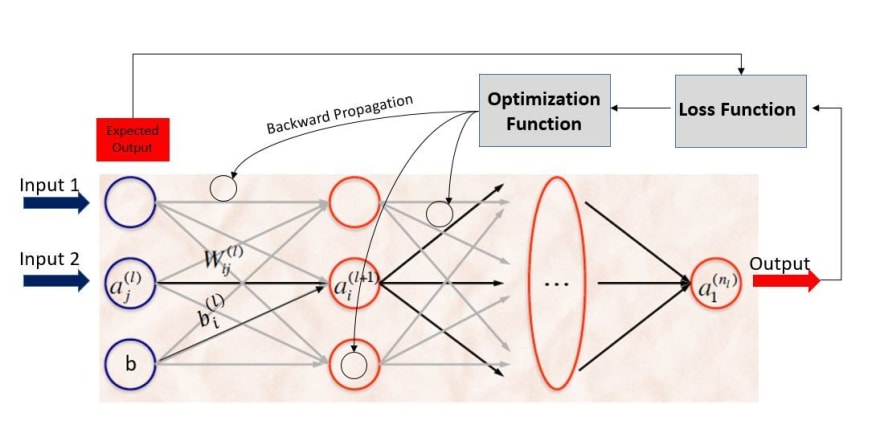
Now that we know what is a ANN and how it works, the last step is to see how it learns. Remember, ANNs are formed by layers of neurons where every neuron is a simple mathematical function whose input term is the sum of the outputs of the previous layer multiplied by some weights and with a bias term added. Figure 10 represents this, where W are the weights, b is the bias term and a is an artificial neuron. The sub indexes "i" and "j" represent the position of the neuron in the layer and the upper index "l" represents the layer in which the neuron is located.

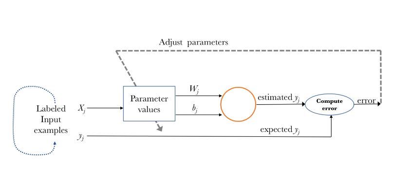
The key to make the ANN learn are the weights and the bias terms. To put it simple, during the process of training we know what the correct output should be. After the ANN made its prediction we can calculate how far away that number is from the expected output. Now we just have to update the weights and the bias term in such a way that the next time the predicted output is closer to the expected one.
Sounds easy right? But how do we do that? We could simply use our intuition, or assign new weights and biases randomly but this probably will not take us anywhere. Instead, we need to define a clear and systematic method of training, which is achieved thanks to the use of the loss and optimization function.
The first step of the training process is the forward propagation where the inputs cross through the input layer towards the output layer. Each time the network outputs a prediction, we compute the difference between the predicted and expected result through the loss or cost function. Once we calculated that difference, we push back this value to every neuron adjusting its weights and bias values in such a way that after each iteration the value of the error obtained is getting smaller. This pushing back process is known as backward propagation and is efficiently performed through the optimization function. The code that makes all this process of training possible is known as the optimization algorithm. Look at figure 11 for a graphical explanation of this.
We could design a simple optimization algorithm. Using the house price example, we can calculate the difference between the predicted price and the real price so we know if the predicted price is bigger or smaller. Now, we divide that difference between the number of neurons at each layer, we multiply the result of this last operation by one parameter and we substract or add this result to the weights and biases. This is one way of updating weights after each iteration but of course, this is not the best way to perform this task. The network may not be able to ever learn anything, or what is the same, the loss functions will not converge to its minimum value at any moment.
The main idea of the optimization algorithm is to make the loss function converge to its minumum after each training iteration. The loss function measures the error, thus, the smaller it is, the smaller the error is, therefore, better is the prediction.
This is the reason why optimization functions usually calculates the gradient of the loss function. The gradient is the partial derivative of the loss function with respect to the weights. After, the weights are modified in the opposite direction of the calculated gradient. Ass we see in figure 12, the gradient vector of one function at a point (x, y) points towards the direction of the greatest rate of increase of the function at that point. If we want to reduce the function, we should move in the opposite direction. Have a look here for more information about gradients.
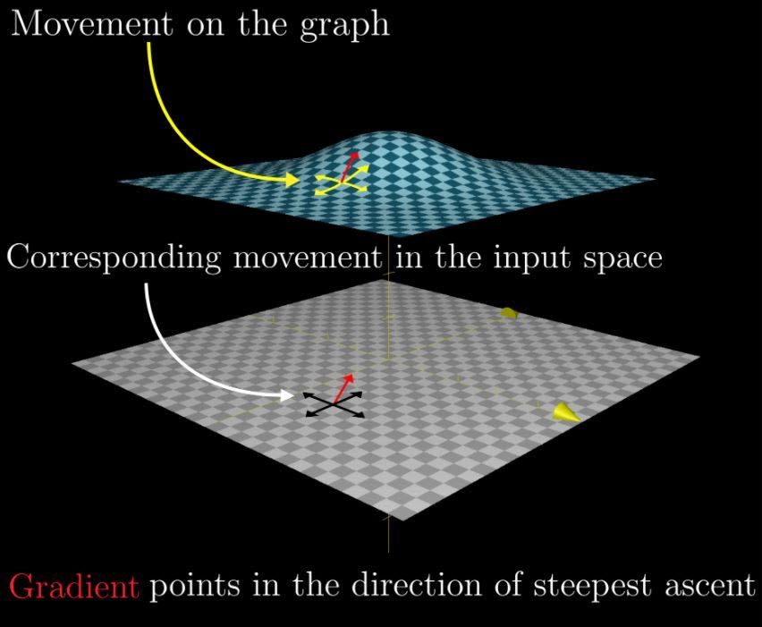
So we calculate the gradient of the loss function with respect to the artificial neuron weight at every layer and we variate the weights and biases of that layer in the opposite direction of the gradient. The amount which we variate the weights is called the learning rate and is represented as alpha (α).
In function of the outputs we are looking for, we have three main categories of loss functions to choose. Regressive loss functions, used in the cases where the target variable is continuous. Embedding loss functions, when we deal with problems where we have to measure if two inputs are similar or not. Classification loss functions, when we deal with problem where we have to determine what class describes better the input from a set of given classes. I am not going to cover any loss function in this post. Only to give you an idea, the mean squared error is a commonly used loss function which calculates the sum of squared values between our target variable and predicted values. Have a look here if you want to see some examples of loss functions.
As of optimization algorithms, they fall in two classes. Constant learning rate algorithms, which use a constant value for the learning rate and adaptive learning rate algorithms which modifies the value of the learning rate while training. Researches suggested that the Adaptive Moment Estimation algorithm (ADAM) compares favorably to any other adaptive learning rate algorithms. It works with momentums of first and second order, storing an exponentially decaying average of both, past gradients and past squared gradients. On the same way as with the optimization functions, I am not going to cover more about the optimization algorithms because is not the goal of this post, but be free to learn more about them here.
On the third and fourth post of this series, where we'll see practical examples where I will explain with more depth the loss function, optimization algorithm and why did I chose the specific activation function for the neurons at every layer.
Now that we've seen all the components of an ANN and what are them for, I think it's a good moment to review the whole process of building a neural network, so you leave with a clear picture of it.
Review of the whole trainining/learning process
Figure 13 shows us a visual interpretation of the training process of a neural network.
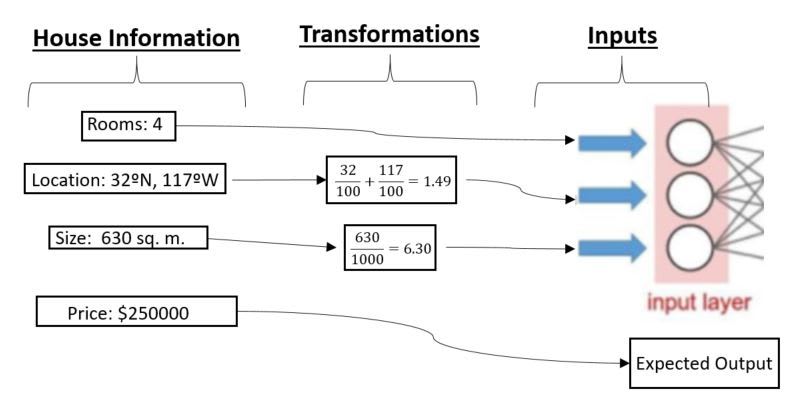
We'll keep using the houses price example. Let's say we have a dataset of 10 thousands homes in San Diego for which we know the price, we know the number of rooms, their size and the neighborhood. As I explained above, the first step is to transform the neighborhood information from text or a map position to numbers. We will use the map coordinates (longitude and latitude) to perform this task and we'll represent both of them as a single decimal number ranging between (-3 and 3). The number of rooms in the house isn't such a big so it should range between 6 and 0, then we could not to apply any transformation to it. Lastly, we will transform the house size information from square meters or feets to a decimal value, so a house of 632 square meters will be inputted as 0.632 to our neurons and a house of 6000 square meters as 6. Figure 14 shows a diagram of this transformations.
At building the ANN you first have to decide how many hidden layers and what kind of neurons you want for each layer. Let's say that we have chose neurons with the sigmoid activation function for the input layer. That's why we did the transformations to the inputs, since the sigmoid has sensibility for an input range of (-6, 6). If we don't transform the inputs to ensure they never get outside that range, our ANN would not be able to consider the house size information nor the location in its predictions, since those values would always be bigger than 6.
Now we have to choose the neurons for the hidden layers. Let's say that we choose the Tanh function for the first hidden layer and the Sigmoid function for the second hidden layer. Remember that the output range for the Tanh function is [-1, 1], and the price of a home is always positive, then the sigmoid on the second hidden layer will transform the output from the Tanh function to a always positive value between 0 and 1. Finally, since the price of a house can vary unexpectedly between the range (0, infinity), we will choose the ReLU activation function at the output layer because we don't want to limit the output between a specific range. What's more, let' say that we want the price to come out of the algorithm in actual dollars, so we don't make any transformation to our expected output.
Knowing that each neuron sums all the input terms and then adds the bias to it, and knowing the input and output range of our chosen activation function, we can assign initial values for the weights and the biases.
In this case, we don't want the input to the first hidden layer to be bigger than 3 or smaller than -3. As the input layer has three sigmoid neurons, each neuron on the first hiiden layer will have a maximum of three inputs that will range between 0 and 1. Then we chose the initial weights value for the input layer to be 1 and the bias term to be 0. Using a similar logic, we set the weights of the first hidden layer to be 1.5 and the bias value as 1.
Finally, since we decided to not transform the expected output, our ANN oputput has to be of the order of several hundred of thousands (the price of a house in dollars). On the second hidden layer we have sigmoid neurons whose output range between 0 and 1. Then we have to set the weights and bias of the second hidden layer in such a way that the sum of all the neurons output is able to result in the price of a house in dollars, because the ReLU neuron at the output will just return the value that it takes as input. Then, we assign weigths of 250000 and a bias term of 100000 to the second hidden layer. Figure 15 shows the distribution that I've commented.

This is a bad distribution. Not normalizing the output was a bad choice, we should have transformed the expected output so we could afford to reduce the weights keeping the network balanced and able to learn at a stable learning rate. For example, to correctly design this ANN we should have tranformed the house price to the order of hundreds or tens. So you can build a scale where the ouput 100 represents a house worth 1 milion.
It make no sense to have such a big weight as 250000. Even if the algorithm would be able to learn, it will progress so slowly, because we have to vary such a big weight with every itteration, that we may not have enough data in all San Diego to make the algorithm learn at the rate it is doing so.
However, I chose to explain it using this bad design to make you understand that the values of the parameters and the types of neurons that are used is the choice of the developer, and there are an infinite number of combination. Of course, you can do whatever you want, but it does not mean that what you are choosing to do works. Only testing and experience will give you the ability to make the right choices.
After we have designed the artificial neural network and initialized the weights and biases, we input the information of our first home from the dataset. Forward propagation process starts and the ANN outputs a value which is the predicted price for the house whose characteristics are given as inputs.
Let's imagine the output is 100000 while the real price is 250000. We use the optimization algorithm to first calculate the value of the loss function and then the gradient of the loss function regarding the weights at each layer. We apply the learning rate to every weight and bias, adding or substracting, whatever is the opposite direction of the gradient.
After this, we input the information of the second home in our dataset and so on and so forth till we have used all the 10 thousands homes from our dataset. Each time we have iterated once with every house from the training set, we completed what is known as an epoch. An epoch is the term that defines the process of training the algorithm once with the full testing dataset. We usually perform several epochs over the same dataset when training an ANN.
We have two ways of visualizing if the training is going well. We could see that the value of the loss function is decreasing at every iteration, and we also could see that the predicted price is getting closer to the expected price at each iteration. Usually, since the value of the loss function can be normalized, tracking the loss function is a better way of monitoring the training process.
Final Thoughts
By now I hope you completely understand what is Deep Learning and how does it works. You should also have a vision about how to choose the appropriate types of neurons and how important is the quality and processing of the dataset. For example, it may be a better option to divide our housing price prediction algorithm in two, one for luxury homes and one for median household owners. In this way we would have a smaller range of inputs and outputs, making it easier for the model to learn, or what is the same, for the loss function to converge at a minimum value. However, it also depends on the application and the client you are developing for.
Another key idea that I want to share about deep learning is that to develop a good model you need a wide knowledge about the problem you want to solve, and you need to understand pretty well the data that you have access to and what can you do with that data. Before deep leaning we had to build the logic of the algorithm in order to predict the price of the house. Now, the logic is automatically learned by the algorithm, but you need to help him do so by defining the correct hyperparameters and preprocessing the data, ensuring it is of high quality. Its like you need to guide the algorithm through the learning process.
By the way. In deep learning we call hyperparameters to every parameter whose value is external to the model and cannot be estimated from the data, (number of hidden layers, number of neurons per layer, activation functions, loss functions, optimization function, optimization algorithm, learning rate, number of epochs at training, etc). We call model parameters to every parameter whose value can be learned by the model during the training process or can be estimated from the data (weights, biases, input/output range, error, etc).
Finally, I want to comment that there are some important aspects of deep learning that we haven't covered. Like overfitting, meaning that we trained the algorithm too many times with the same dataset so it performs almost perfectly for any given value form that dataset but it fails at predicting when a value outside that dataset is inputted. Also, when we have a dataset of values, we have to be sure that the values inside represents all the possible options. For example, if we have an 80% of medium class houses in the data, our model performance will be low when predicting the price of a luxury home. Furthermore, we need to track the performance of our model after training, so we don't use all the data that we have in our database for training. We split the dataset between the training set and the testing set, ensuring that both sets contain examples from all the possible values.
We will cover this concepts in the third and fourth posts, where I will share with you two practical examples of this, using python.
The next post, coming out in approximately a month, will be about the different types of artificial neural networks and what are them most suited for.
Thank you !!


Top comments (1)
Totally agree Rosie,
Another interesting factor would be to create an open source global data-set for every application. Let's suggest autonomous driving.
For just one car-maker it is extremely hard to build a data-set including every possible real life driving occurrence. Instead, if we have an open source data-set where all the self driving car-makers upload their use-cases and examples, then any car maker would be able to use that data to train it's vehicles.
It will become cheaper to train your cars (you don't need to pay a driver and build cars just to go all around), and it also would become easier to train cars for driving in different countries and scenarios.
However, easy to say but hard to do. It is expensive to drive cars around just to upload the information to a data lake accessible to everyone. We could install cameras on people cars and use that information for training, nonetheless, privacy and data regulations "GDPR" must be considered here.
There are many ethical, political and monetary interests that slows down AI implementation in many technologies. But no worries, step by step society is solving those conflicts, and AI will be soon implemented to manage data flows in most of the industries.
I recommend watching (Third Industrial Revolution Documental by VICE): youtube.com/watch?v=QX3M8Ka9vUA&li...
BTW: Merry Christmas !!