Hi all,

This is the second post of the series Deep Learning for Dummies.

Below you have the lists of posts that I plan to publish under this series. I will keep it updated with each published post. Unpublished posts titles and used libraries can change:

1. Introduction to Deep Learning, basic ANN principles
2. Artificial Neural Networks: types, uses, and how they work
3. CNN Text Classification using Tensorflow (February - March)
4. RNN Stock Price Prediction using (Tensorflow or PyTorch) (April - May)
5. Who knows? I may extend it. Perhaps some SNN use case.

In this post you'll learn about the different artificial neural networks, how do they work, and what is each type most suited for. This is still going to be a fully theoretical post with no code involved. No worries, next posts are going to be fully practical. We'll apply all the concepts learned in the introduction post and use one of the neural networks in this post to solve real-life use cases.

Table of Contents

Let's go with the table of contents that we'll cover:

• Introductory Concepts
• Artificial Neural Networks
• Convolutional Neural Networks
• Recurrent Neural Networks
• Spiky Neural Networks
• Final Thoughts

Introductory Concepts

The most complete topologies guide for the different types of artificial neural networks used in deep learning can be found here. I encourage you to have a look since you can also see a short description of what each one is suitable for.

In deep learning, we classify artificial neural networks based on the way they operate. Then, as we'll see through this post, all the artificial neural networks used currently in production fall under four main categories, artificial neural networks (ANNs), convolutional neural networks (CNNs), recurrent neural networks (RNNs), and spiking neural networks (SNNs).

Artificial Neural Networks

It may seem confusing since all the neural networks used in computing are artificial neural networks, however, we reserve this definition for all the neural networks that are distributed in several layers of artificial neurons and only performs the operations of those neurons to obtain the output.

The neural network used as an example in my previous post where I explained how to do the house prices estimations, was an ANN. The typical structure of those neural networks can be seen in figure 1.

As you can see. We have the inputs to the neural network, which is always formed by a set of numbers, we have the input layer, the hidden layers, and the output layer. That is the structure of an artificial neural network "ANN". In my previous post I explained how this works, so let's switch to the next type, the CNN.

Convolutional Neural Networks

The name of this type of artificial neural network comes from the two operations that they perform over the inputs before feeding them to one usual ANN. Those two are the convolution and pooling operations. Before zooming into what are them, see a graphical representation of a CNN in figure 2.

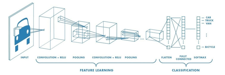
Most usually CNNs are used for image processing, that is why the input is the figure is an image. As we can see, the first and second layer is a convolutional layer and a pooling layer respectively. Those came hand in hand with each other, which means that every time we insert a convolutional layer we have to insert a pooling layer afterward. We could insert as many convolution-pooling layers as we want, of course in reality it will depend on our application and the size of the input. The output of the last convolution-pooling operations will be a matrix of numbers. This matrix is converted into one vector which is called the flatten vector, thus sometimes you will hear the name flattened layer. The flattened vector is afterward inputted to a fully connected layer which is just a layer of ANN neurons as we saw in the previous post. Lastly, we have the output layer which provides the prediction. Now let's see what the convolution and pooling operations mean.

Convolution operates on two signals (in 1 dimension) or in two images (in 2 dimensions). We could think of the first signal as the input and the second signal, called the kernel, as the filter. Convolution takes the input signal and multiplies it with the kernel, outputting a third modified signal. The objective of this operation is to extract high-level features from the input.
There are two types of results. Where the output is reduced in dimension (this is called Valid Padding) and where the output has the same dimension or even bigger (this is called Same Padding).

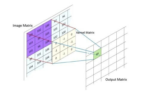
Figure 3 shows an illustration of the convolution operation. An image is nothing else than a matrix full of pixels, the convolution operation consists of passing a filter (the kernel matrix) through the image matrix, this means that the kernel matrix slides step by step, one position in every direction, over the image matrix. It multiplies each image matrix cell value by the cell value in the kernel matrix, sums all the obtained values, and stores the result in the respective cell of the output matrix. The weights of the kernel matrix are initialized by default to some value and are updated through the training process.

The idea of the convolution operation is to mimic the human eye detecting features in one image. When we see a car image, there are some features in the image that makes us recognize there is a car (shape of the car, material, roads, intersections, etc). Multiplying the image matrix by a filter and updating the
filter parameters through training extracts the most important features of the image, those that make us understand a car is in the image but we don't know how to detect algorithmically.

Figure 4 shows an illustration of the pooling operation. It is a sample-based discretization process where we down-sample an input reducing its dimensions and allowing for assumptions to be made about features contained in the selected sub-regions. This is done to decrease the computational power required to process data while extracting dominant features. There are two main types of pooling operations. Max pooling of which we can see a graphical representation in figure 4 and average pooling. As their name suggests, one of them is based on picking the maximum value from the selected region while the other is based on calculating the average of all the values.

The output of the last pooling layer in a CNN is a multidimensional matrix named pooled features map. We need to flatten this final output into a vector containing one value per index to be able to feed it to the fully connected layer, this is the flattened vector represented in figure 5. The features filtered through the convolution-pooling steps are encoded in the flatten vector. The role of the fully connected layer is to take all the vector values and combine features in order to make a prediction about the probability of each class.

Just as a side note, when working with color images there are three matrixes, one per color (Red Green Blue "RGB"). Then, we will have to work with three matrixes separately. In addition, one filter (or kernel) may not be the most adequate to extract all the features from the image. This is, in one portion of the image a filter with a specific length and parameters is most adequate while in other portions of the image another dimension and parameters may be better to properly extract the features. Thus, when applying the kernels over one image we will apply several kernels at once and each with different dimensions and different initial parameters. We'll see more about this in the next post, where we will use a CNN to predict text sentiments.

Obtaining the correct number of kernels and their size, as well as the correct pooling operation can be achieved only through practice. Another important factor is that we must be coherent with the images dataset that we are feeding the CNN. If we train a CNN to differentiate between terrestrial vehicles, but not planes, then don't introduce a plane image in your training set.

Why? Because the final output of a CNN represents the probability of inputs belonging to a specific class. When training we'll feed the CNN with photos of trucks, tractors, vans, and cars. Each of these vehicles represents a class and we'll correct the CNN each time it predicts that a vehicle is in a class it does not correspond. Sames as ANNs, through backpropagation, fully connected layer weights and parameters in the kernel matrix are updated, so the CNN learns how to predict which class is each vehicle. If you have a plane image in your training set and there is no plane class at the output, all you're doing is to worsen the parameter updating process. The CNN will associate features of a plane with another vehicle class.

Since CNN outputs are probabilities of the input to belong to each class, the sum of all outputs will always range between 0 and 1. If you use the trained CNN to differentiate between vehicles and you input an airplane image, in the best case scenario the four classes output may be 0.25 (meaning that the input hast the same probability of belonging to any class). If this is the case then you can detect that the input belongs to none of the four classes. But it is also possible that the CNN outputs a higher probability for one of the classes, so you may wrongly consider that there is a truck where in fact is an airplane.

Recurrent Neural Networks

This type of neural networks are ANNs designed in an algorithmic way that gives the network the ability to perform time analysis predictions. This means that we can work with inputs where the sequence of the input matters. For example language translation, text generation, or stock price prediction.

The order of the words in a phrase does matter, it is not the same to say "I have to read this book" than "I have this book to read". RNNs are used by the popular google translator, RNNs suggest you the next word when typing an email and they even suggest you a new easy reading and grammatically correct structure for the entire sentence, if you ever used Grammarly. So let's see how it all works.

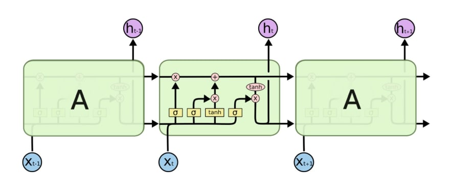
Figure 6 represents a Recurrent Neural Netowrk. In order to process time series inputs and predict "ht", apart from the actual time input "Xt", RNNs use a new variable, called hidden variable or hidden state, whose value depends on the previous prediction when the input was "Xt-1".

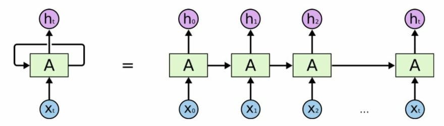
The rectangular block "A" represents a usual ANN, with its input layer, hidden layers, and output layer. The loop arrow over block "A" represents the usage of information from previous predictions at predicting the current output. The right side of the equal symbol is a breakdown of the time series prediction process. Let's suppose we want to predict the stock price for the next week (Monday to Sunday) based on the sales perspectives announced by the company for that week. X0 to X6 are the inputs representing the expected sales at day one, day two, and so forth till day seven. Similarly, h0 to h6 represent the stock price predicted for day one to day seven respectively.

First, the ANN takes as input X0 and predicts the stock price for Monday "h0", during this prediction the value of the hidden state or hidden variable (both terminologies are used) is updated. This variable, together with Tuesday "x1" sales information, is used to predict the share price for Tuesday "h1". Meanwhile predicting the stock price, the hidden state (or hidden variable) is updated and then used in the prediction of "h2". This loop is maintained till the RNN performs the prediction of all seven days of the week.

Note that hidden state refers to a concept totally different from hidden layer. A hidden layer is a layer of artificial neurons enclosed between the input layer and the output layer.

Hidden State or Hidden Variable is just another input to the ANN which is calculated based on the predictions at previous time steps in the sequence. This is the way we can store the sequence information up to step "t-1", it gives the concept of memory to the RNN. The value of the hidden state at time "t", is calculated based on the input at time "t" and the value of the hidden state at time "t-1".

There are two common approaches to defining and updating the hidden states, depending on the problem. If the problem is that of contiguous sequences (for example working with text which is always about the same topic) then the hidden state of the next sequence is the last version of the hidden state in the actual sequence, this is, the hidden state is initialized once randomly and that initial value is being updated during all the training process. The other approach, used when working with distinct sequences (random tweets as an example), consists of initializing the hidden state with the same value each time we start predicting a new sequence.

Hidden states are updated through backward propagation using weights, those weights are what the RNN stores and uses to update the hidden state value at performing predictions in production.

As seen in my previous post, we use the gradient of the cost function to update the weights in a process which is called backward propagation. The backward propagation process is problematic for the RNNs because of the vanishing/exploding gradient problem.

Imposed by the structure of the RNN, information from every previous step is used when updating the weights at any given time step. If we make a mistake at updating the first steps, that mistake is going to be passed to the next steps and it will be worsened because of derivatives properties. If we mistake by updating to a lower value than needed, at each next step the updated value will be even smaller than needed, resulting in a vanishing gradient. In contrast, if we mistake by updating to a bigger value, the value will become bigger than needed each time step in the series, resulting in an exploding gradient. This prevents our RNN from learning. Figure 7 below is a summary of this problem.

There are different ways of solving this vanishing/exploding gradient problem, however, for the sake of the length of this post and because it is the most used in practice I am going to shortly explain the long short term memory "LSTM".

Long Short Term Memory consists of giving a specific structure to the ANN present in the RNN. This specific ANN consists of 4 layers of neurons interacting between themselves. Figure 8 is a representation of the LSTM showing us the structure of each ANN, "A", in the figure.

The LSTM adds the new concept of cell states which gives the model longer memory of past events. Its function is to decide what information to carry forward to the next time step. This is achieved thanks to the combination of several steps. Have a look at figure 9 below. There are three entries to the ANN in one step, the input, the hidden state, and the cell state. First, by what is seen in the figure as "ft" (forget function) the RNN decides if to forget the information coming from the previous step or not. After, through what is seen in the picture as "Ct", it computes what information from the actual step should be carried to the next time step and adds that information to the cell state variable. Lastly, it computes the output and the hidden state.

To explain a practical use of this architecture. Let's say that we are translating the phrase "Adrian is being late", then when translating the first word, "Adrian", we store it into the cell state and send that information to the next steps, this way the RNNs can remember the subject of the phrase at translating. This is useful if, for example, in some language the correct structure is to put the subject at the end. So instead of "Adrian is being late" the translation should write "Is being late Adrian".

We'll end the RNNs explanation here. In the 4th post of this series I'll implement a simple stock prediction algorithm using this kind of neural network. We'll go into further detail about practical examples in python then.

This post is being already longer than I expected, nonetheless, I recently discovered a totally new concept of artificial neural networks which really intrigued me, so I would like to give you a brief overview about what are those, the Spiking Neural Networks.

Spiking Neural Networks

SNNs have been developed for neurological computing in an attempt to model the behavior of the biological brain. It seems that they have been around for a while, but have not sparked up deep learning interests mainly due to a lack of training algorithms and increased computational complexity. SNNs mimic more closely the neural connections in our brain, thus they are the most bio-inspired artificial networks created till the present.

Figure 10 is a representation of two biological neurons, our brain is made out of billions of these interconnected to each other. They use the axon terminals to transmit signals while the dendrites are in charge of receiving signals. From an engineering point of view, neurons work by transmitting and receiving electric spikes between them. This is, they produce a voltage increased for a short period of time and then it gets back to its neutral status. Biologists do not agree with this description because it is very primitive, however, it is a practical simplification and it works for computational brain modeling. Here you have a long series of videos from Khan Academy explaining the brain's functioning from a biological perspective. In the next paragraph, we'll briefly cover the concepts we need to later understand how a SNN neuron works.

Each receptor in our body (eyes, nerves, ears) activates one or several neurons with electrical impulses. The impulse is received by the neuron's receptive field and it needs to surpass a threshold value in order to activate the neuron. When this threshold is activated we say that it fires an action potential. Each neuron in the nervous system has its own receptive field threshold limit, meaning that impulses which activate one neuron may not activate another one.

The action potential travels along the neuron, reaching the axon's terminals, where it causes the release of neurotransmitters. Those neurotransmitters travel and attach to the dendrites of another neuron, which is the receiver. There exist several types of neurotransmitters in our brain, and the effect they have on the neuron depends on their type. Biological neurons are connected with thousands of other neurons, then they can receive different neurotransmitters at the same time. The combination of the received neurotransmitters determines neuron behavior.

When the amount of neurotransmitters received by a neuron surpass a certain threshold value, the equilibrium of the neuron changes and triggers the action potential, which travels to the axon terminals and produces the discharge of neurotransmitters. Each neuron contains a different amount of neurotransmitters in its axons, thus, the more neurotransmitters it has, the more it transmits, the stronger is its influence over the receiving neuron. On the same way, some neurons dentrites are more prone at receiving neurotransmitters than others. Those factors determine the strength of the connection, meaning that a neuron does not have the same influence over all the other neurons it is connected with, and, a receiving neuron is not influenced equally by all the transmitting neurons it is connected to. Just for general knowledge, transmitting neuron is called presynaptic neuron while the receiving neuron is called postsynaptic neuron.

Now that we have the basics about how does our brain transmit signals, we can understand how SNNs works since it is an analogy. In figure 11 you can see that the structure of an SNN is different from those we have used for ANNs, CNNs and RNNs. The layers concept is lost and neurons are multiple-connected between each other forming a mesh. This emulates the way neurons in our brain are connected, being this the reason why SNNs are the correct tool to use at studying biological brain behavior.

I guess you heard about Elon Musk open AI company. Well, they are testing the implementation of chips to read and transmit signals to our neurons. Another important fact, a group of researches have achieved the control of a bio-inspired robot insect "RoboBee" through the usage of an SNN, while the Cortical Labs team in Australia have developed silicon chips combined with mouse neurons. If Yuval Noah Harari in his trilogy (Sapiens, 21 Leesons for 21 Century, Deus) is right and the evolution of homo-sapiens goes towards cyborgs, then it looks like SNNs are part of this transformation.

To mimick the way biological brains work, Spiking Neural Networks neurons must be defined in such a way that they can be activated asincornosly and shoot pulses as output. ANNs are not accurate models of the brain because layers are activated synchronously and they used continuous-valued activation functions. Each neuron outputs a continuous value. In our brain, after the action potential happens and the neuron transmits the neurotransmitters, it then passes back to its stable state, waiting for the next activation.

Several techniques can be used to emulate such a behaviour, but one of the most used and easy to understand is to use the Leaky Integrate and Fire (LIF) model to represent neurons.

Under the Leaky Integrate and Fire (LIF) model, neurons are represented as a parallel combination of a resistor (R), a capacitor (C) and a switch. See a graphical representation in figure 12. A current source (Idc) is added to represent the biological neuron activation impulse. First, the current source charges up the capacitor, which produces the potential difference Vc.

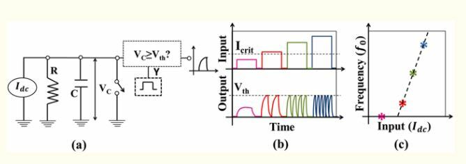
Part b) of the above figure shows the graph which represents the neuron output based on the current input Idc. We can see there is a threshold current input "Icrit" below which the neuron's output voltage "Vth" never reaches the threshold voltage "Vth". If at any given moment the input current "Idc" is bigger than the threshold current "Icrit", then the neuron output reaches the threshold voltage "Vth". Reaching "Vth" triggers the switch discharging the capacitor, so we see an immediate decrease of the voltage "Vdc". This discharge produces a voltage pulse that is called a spike. The spike's shape comes from the natural charging-discharging cycle of the capacitor. Have a look here to understand what and why a capacitor's charging-discharging cycle produces spike looking pulses.

This spike emulates what the biological neuron does when is activated through stimuli, the neuron receives neurotransmitters from thousands of others till its equilibrium is unbalanced (till the threshold "Icrit" is surpassed). This produces the action potential which discharges neurotransmitters over another neuron and it goes back to equilibrium waiting for next activation (the process of transmitting and getting back to equilibrium is represented by the capacitor charching and discharging cycle).

We've commented that there exist different neurotransmitters and their combination change neuron behavior. We emulate the transmission of different neurotranmsitters through the output frequency.

Frequency is defined as the number of waves that pass a fixed point in a unit of time. We can see in the output graph that at a bigger current input "Idc", bigger is the output frequency. Look at the red spikes, green spikes, and blue spikes. The bigger is Idc at the input, the more waves we have at the output Vc. Then based on the input, we can have different outputs. In addition, increasing or decreasing the threshold values for Idc and Vc we emulate different strength of connections. This can be achieved by changing the resistor resistance and capacitor capacity.

Then, this is how we simulate a biological neuron. Now we have to connect them between each other forming a mesh. How do we do that?.

Figure 13 represents how a connection between two LIF neurons works. First, D1 and D2 are two drivers that control the voltage input to the neuron. In this case, two neurons are connected to the receiving one and they are transmitting two different neurotransmitters (spikes at different frequencies). W1 and W2 are where the input voltage spikes are transformed to a flow of current. Those two currents are summed and they flow towards the "N3" neuron capacitor. If the input current is bigger than the threshold value, the output voltage produced by the capacitor will also be bigger than the threshold voltage. The switch activates and the capacitor discharges creating the spike shape output. This output is received by the output driver "D3" which converts the analog spikes response into proportional voltage pulses whose values depend on the frequency and intensity of the spikes. Those last pulses are the input to another neuron.

So we reached the point where we know how spiking neural networks are formed. But we still don't know how it works. How do they learn?. Backward propagation isn't valid anymore because in order to calculate the gradient descent you need to define a continuous variable for the output, and spikes are not like that.

Till present, SNNs have been used in computational neuroscience as an attempt to better understand how our brain is functioning. One really interesting and active field of investigation is neuromorphic engineering, where we design computers implementing physical hardware level SNNs to perform tasks of the biological nervous system.

For example. If you want a robot to go to a certain position based on the camera lecture, you need to implement a program detecting all the objects (perhaps use a CNN for this), calculate the adequate route (this is achieved by state-space representation and heuristic searches), activate the wheels based on that calculated route and so on. All this system is implemented over classical hardware architecture, where sensor outputs are stored in memory same as the algorithms and programs. All the information is processed by a CPU and several integrated systems which then dictates what actuators have to do, like moving the wheels at a certain angular velocity.

With neuromorphic engineering, we will have a device (computer) where physical spiky neurons are implemented with the use of oxide-based memristors, spintronic memories, threshold switches, and transistors. Sensors and actuators may be directly connected to this device and then the SNN trained to activate the actuators based on the outputs of the sensor. No more memory-cpu-controllers-integrated circuits connection needed.

The main benefit of neuromorphic devices is energetic efficiency, since information can be transmitted through the neural network using very weak signals.

Now the big questions. How does this SNN work? How do we train it? How and why does it learn?

I want to be honest here and let you know that I still don't know exactly how they do it, so I am not able to explain step by step what happens at each learning phase. However, I will shortly share some interesting information about this.

To make Spiking Neural Networks learn we have to use unsupervised learning algorithms, this is, to let them learn by themselves. Some bio-inspired used learning algorithms are Hebbian Learning or Spike Time Dependent Plasticity. These rules enhance the weights of the receivers (W1 and W2 in figure 13) if the activity of the connected neurons is correlated, and decrease if the activity is not correlated. Therefore, the strength of the connection is higher for neurons that perform related activities. A stronger connection means that the transmitting neuron has a bigger impact on the receiving neuron. Let's suppose the SNN has trained already. When an input is received, the path of the spikes is determined by the strength of the connection. With the training process, we modify the strength of the connection to activate the same path of neurons when a similar input is given. Then, no matter if a car, a rock or any other object is dangerously approaching. In both cases same path of neurons will be activated and the action would be to esquivate. We eliminate all the processing power of detecting the object, identify the danger, calculate an escape path, etc. In fact, we don't eliminate that process, is just that the SNN has learned it automatically, without us having to define all those steps. However, this technology is very underdeveloped. There's still a lot of work to do to achieve desired results.

Recently (in 2020), it has been implemented a fully neuromorphic optical platform able to recognize patterns learning by itself.

Final Thoughts

This post is longer than I expected. The most accurate and sincere final tough ever :D

Anyway, the main reason is the explanation of the Spiking Neural Networks which I believe are the most interesting of all. They are not widely known by most programmers since are not implemented in deep learning algorithms, so I've encountered many AI courses, blogs, articles where SNN are not even mentioned.

The next two posts will consist of practical implementations of CNN and RNN. In the third post, we'll see how to implement a CNN for text classification while in the fourth post we are going to see how to perform stock price prediction using RNN. In both cases, I am going to use python and the TensorFlow library.

Below, you can see a video simulating the different Neural Networks activities. It's just three minutes long. I recommend watching.

Image is just a link. It will redirect

If you have any suggestions, doubts, don't hesitate to use the comments. We are all here to learn and share our knowledge. And, don't forget to follow me on LinkedIn and/or Twitter.

Thank you !!!