
Implementing Linear Regression and Statistics on a Parking Lot Dataset to advice the city based on the Regression Lines and Analysis regarding the enlargement of the Parking Lots.
The dataset can be downloaded from the following link:
https://github.com/ruthvikraja/Parking-Lot-Dataset.git
Prior Knowledge about the Dataset and the Goal of this Article:
A city is planning to improve the performance of some Parking Lots. The city provides the occupancy of each Parking Lot for around three and a half years. So, the goal is to Rank the Parking Lots necessity for enlargement from the most to the least urgent. [Assume that the Parking fees of all the Parking Lots are equal]
The Python Code is as follows:
import matplotlib.pyplot as plt
import seaborn as sns
import pandas as pd
import numpy as np
from sklearn.linear_model import LinearRegression
df=pd.read_csv("/Users/ruthvikrajam.v/Desktop/ML/Parking_lots_dataset.csv")
df.info() # Check if there are any null values in the data set
# Let us separate the input data into 5 different dataframes based on the parking lot number
df1=df[df["Parking Number"]=="Parking lot 01"]
df2=df[df["Parking Number"]=="Parking lot 02"]
df3=df[df["Parking Number"]=="Parking lot 03"]
df4=df[df["Parking Number"]=="Parking lot 04"]
df5=df[df["Parking Number"]=="Parking lot 05"]
## df1
x=np.array(range(df1.shape[0])).reshape(df1.shape[0],1) # The shape displays the number of rows and columns in a Dataframe
y=df1.iloc[:,2].values.reshape(-1,1) # Selecting all the rows in 2nd column and reshaping it to fit the values in Linear Regression class
lr=LinearRegression() # creating object for linear regression class
lr.fit(x,y) # fitting the values
y_pred=lr.predict(x) # predicting the output values
plt.figure(figsize=(20,10)) # Since the count of x values is very high, defining the size of the figure to avoid overlapping in y values
plt.scatter(x,y)
plt.plot(x,y_pred,color="red")
plt.xlabel("Number of Days")
plt.ylabel("Occupancy")
plt.show()
df1.describe()
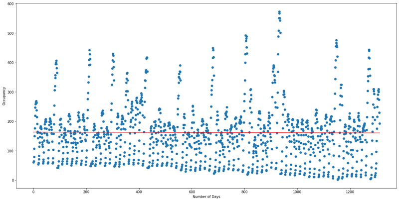
# On an average only 162 are filled out of 577 means only 28%
# 50% of the data is less than 157 means 50% of the days is filled with more than 27.2% occupancy
## df2
x=np.array(range(df2.shape[0])).reshape(-1,1) # The shape displays the number of rows and columns in a Dataframe
y=df2.iloc[:,2].values.reshape(-1,1) # Selecting all the rows in 2nd column and reshaping it to fit the values in Linear Regression class
lr=LinearRegression() # creating object for linear regression class
lr.fit(x,y) # fitting the values
y_pred=lr.predict(x) # predicting the output values
plt.figure(figsize=(20,10)) # Since the count of x values are very high, defining the size of the figure to avoid overlapping in y values
plt.scatter(x,y)
plt.plot(x,y_pred,color="red")
plt.show()
df2.describe()
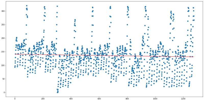
# On an average 136 are filled out of 317 means 42%
# 50% of the data is less than 135, here the mean and median values are almost equal this means
# that the data is equally distributed from lowest to highest values i.e from 0 to 317
count1=df2[df2["Occupancy"]>=317].count()
print(count1[-1]) # Total % of days with more than the total capacity is just 4%
## df3
x=np.array(range(df3.shape[0])).reshape(-1,1) # The shape displays the number of rows and columns in a Dataframe
y=df3.iloc[:,2].values.reshape(-1,1) # Selecting all the rows in 2nd column and reshaping it to fit the values in Linear Regression class
lr=LinearRegression() # creating object for linear regression class
lr.fit(x,y) # fitting the values
y_pred=lr.predict(x) # predicting the output values
plt.figure(figsize=(20,10)) # Since the count of x values are very high, defining the size of the figure to avoid overlapping in y values
plt.scatter(x,y)
plt.plot(x,y_pred,color="red")
plt.show()
df3.describe()
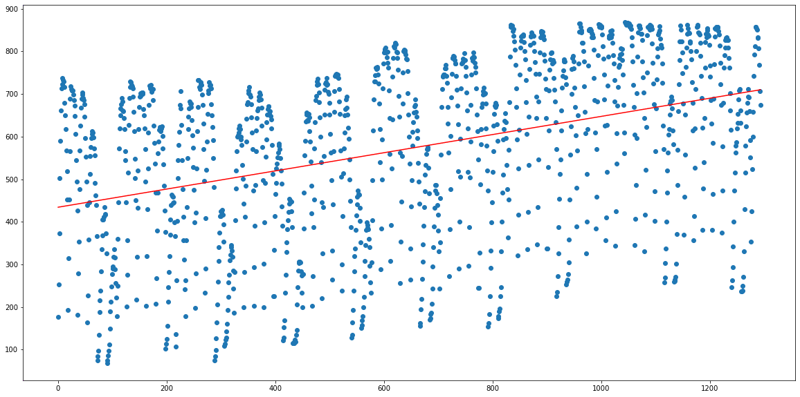
# On an average 572 are filled out of 863 means 66%
# The median of the data is less than 618 i.e 50% of the days are filled with more than 72% occupancy
count2=df3[df3["Occupancy"]>=863].count()
print(count2[-1]) # Total % of days with more than the total capacity is 11%
## df4
x=np.array(range(df4.shape[0])).reshape(-1,1) # The shape displays the number of rows and columns in a Dataframe
y=df4.iloc[:,2].values.reshape(-1,1) # Selecting all the rows in 2nd column and reshaping it to fit the values in Linear Regression class
lr=LinearRegression() # creating object for linear regression class
lr.fit(x,y) # fitting the values
y_pred=lr.predict(x) # predicting the output values
plt.figure(figsize=(20,10)) # Since the count of x values are very high, defining the size of the figure to avoid overlapping in y values
plt.scatter(x,y)
plt.plot(x,y_pred,color="red")
plt.show()
df4.describe()
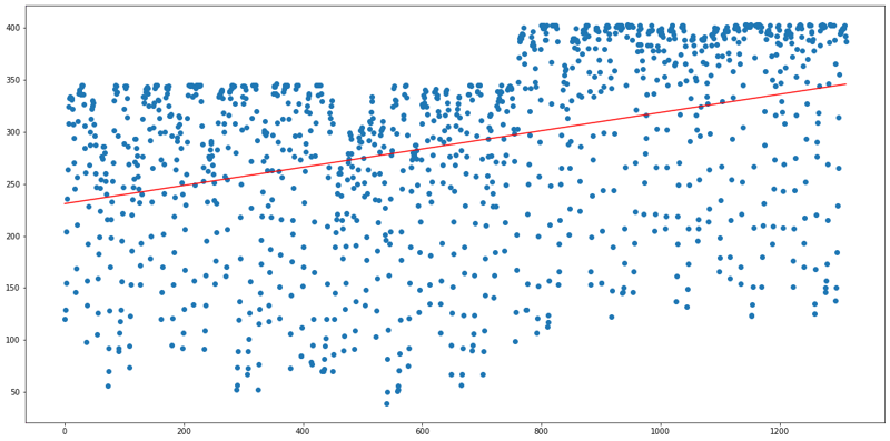
# On an average 288 out of 387 are filled means 74%
# The median of the data is less than 309 i.e 50% of the days are filled with more than 80% occupancy
# The max capacity is 387 but the max value for occupancy is 403 this means that there is a need for enlargement
count3=df4[df4["Occupancy"]>=387].count()
print(count3[-1]) # Total % of days with more than the total capacity is 19%
## df5
x=np.array(range(df5.shape[0])).reshape(-1,1) # The shape displays the number of rows and columns in a Dataframe
y=df5.iloc[:,2].values.reshape(-1,1) # Selecting all the rows in 2nd column and reshaping it to fit the values in Linear Regression class
lr=LinearRegression() # creating object for linear regression class
lr.fit(x,y) # fitting the values
y_pred=lr.predict(x) # predicting the output values
plt.figure(figsize=(20,10)) # Since the count of x values are very high, defining the size of the figure to avoid overlapping in y values
plt.scatter(x,y)
plt.plot(x,y_pred,color="red")
plt.show()
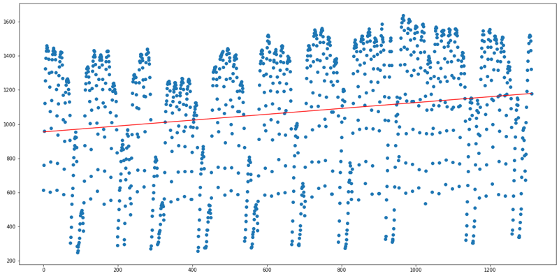
df5.describe()
# On an average 1067 are filled out of 1920 that is 56%
# The median of the data is less than 1162 i.e 50% of the days are filled with more than 61% occupancy
The Regression Plots for the above Python Code are as follows:
X axis —-> Number of days
Y axis —-> Occupancy
df1(Parking lot 01):
df2(Parking lot 02):
df3(Parking lot 03):
df4(Parking lot 04):
df5(Parking lot 05):
Thereby, ranking the Parking Lots for immediate enlargement as follows:
From the above Regression plots, it is clear that Parking lot 04 requires an immediate enlargement because it has high demand as the regression line is increasing drastically, on an average 74% of the occupancy is getting filled and 19% of the total number of days is getting filled by vehicles with more than its maximum capacity.
Then comes Parking lot 03 because it is also having high demand that can be visualised from the regression plot, on an average 66% of the occupancy is getting filled and 11% of the total number of days is getting filled by vehicles with more than its maximum capacity.
Then comes Parking lot 05 because from the regression plot it is clear that there is slight demand for parking, on an average 56% of the occupancy is getting filled and 50% of the days are getting filled with more than 61% occupancy.
Then comes Parking lot 02 with an average occupancy of 42%, 50% of the days
are getting filled with more than 42% occupancy and only 4% of the total number of days are getting filled by vehicles with more than its maximum capacity.Finally, the least preference can be given to Parking lot 01 because the demand is less, the regression line is also constant and the average occupancy is also very low.


Top comments (0)