It is an image enhancement technique.
It represents frequency of occurrence of various grey levels that are present in an image.
It produces visually pleasing results out of noisy or dark images.
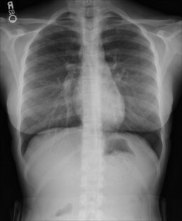
Input image[2^8 bit image]:
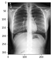
Output image:
import matplotlib.pyplot as plt
import cv2
import seaborn as sns
import numpy as np
img=cv2.imread("/Users/ruthvikrajam.v/Desktop/X-ray.jpg",0)
# Importing a greyscale image in 2D so 0 is passed as a parameter
plt.imshow(img, cmap='gray') # Displaying an opencv image using matplotlib
plt.hist(img,bins=20) # Plotting an Histogram for the Input Image
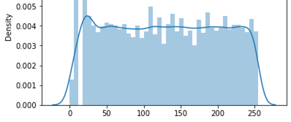
sns.distplot(img) # Plotting KDE of an image, the intensity values are not equally distributed
x=img.flatten() # The Flatten Image command merges all of the layers of the image into a single layer with no alpha channel
hist, bins= np.histogram(x,256,[0,256]) # 256 is no of bins, [0,256] means range which sets lower and upper range of bins
# Basically here we are finding the frequency of each grey level image from 0 to 255 and storing the result in hist
pdf=hist/(hist.sum())# Finding the Probability Distribution Function of the input image
cdf=pdf.cumsum() # Finding the Cumulative distribution of all the intensity values in an ascending order[0-255]
cdf_normalized= cdf*255 # Now we have to multiply each value with maximum intensity value of an input image
# Here we can do any other operation also but I have chosen to multiply with the maximum intensity value of an input image
rounded=np.round(cdf_normalized) # since digital image consists of discrete intensity values, rounding off to the nearest intensity value
img1=cv2.imread("/Users/ruthvikrajam.v/Desktop/X-ray.jpg",0)
row,col=img1.shape
for i in range(0,row): # row= 312 # col= 256
for j in range(0,col):
new=img1[i][j];
img1[i][j]=rounded[new];
# Here we are replacing the actual intensity value of each pixel with the rounded intensity value
plt.imshow(img1,cmap="gray") # Modified image
sns.distplot(img)
sns.distplot(img1)
# Compare the KDE for original and modified image
Why after doing histogram equalisation also we won't see a uniform distribution ??
Ans: (1) Histogram equalisation will try to make the PDF as uniform as possible, while at the same time respecting the original properties of the image and (2) we are converting the Continuous CDF values to Discrete CDF values since our output image should contain only discrete intensity values.
This is also another reason why we will not get a perfectly uniform histogram as result.


Latest comments (0)