Create your first machine learning model in 5 minutes with Google Colab

Machine Learning is a very hot topic these days. Companies from different sectors and sizes, from startups to enterprises, are boosting their products and services with the help of machine learning.

As the demand for machine learning engineers grows, many experienced developers want to get to the field as fast as they can.

But as soon as they buy their first courses and books, they got frustrated. Instead of code and working examples, they face a bunch of math and statistics, topics that they haven't applied since graduation.

Besides math, another source of frustration is the necessary software to build machine learning models. A few years ago, you had to install specialized software, buy powerful hardware and sometimes implement your algorithms from scratch.

The good news is that none of these is necessary to get started in machine learning. Current machine learning libraries abstract most of the math and algorithms you need so you can concentrate on the data flow instead of implementation details. Also, a web browser is everything you need to start creating your first machine learning models.

In this tutorial, we are going to create our first machine learning model using the most famous Python libraries and the Google Colab environment, so we don't have to waste any time installing and configuring new software.

Google Colab

In this tutorial, we use the Google Colab tool to create Python notebooks. A notebook is a special file in which we can mix formatted text and Python code so we can create a rich documentation for our machine learning experiments. Also, we can plot charts directly to the notebook.

In order to create Python notebooks with Google Colab, all you need is a Google account and to click the link https://colab.research.google.com.

For a quick introduction to the Google Colab environment, watch the video Get started with Google Colaboratory:

https://youtu.be/inN8seMm7UI

Classifying Iris exemplars

In this tutorial we are going to build a machine learning model to determine to which species an Iris flower belongs to. The Iris dataset contains tabular data about characteristics of the flower exemplars like petal width and length, which are used as input to the model. The output will be an integer indicating representing one of the 3 possibilities of species: Iris Setosa, Iris Versicolour or Iris Virginica. The next sections will describe the construction of the model, step by step.

0. Setup

In this section we import the necessary libraries so you can build your model.

import numpy as np
import pandas as pd

from matplotlib import pyplot as plt

import seaborn as sns

from sklearn.model_selection import train_test_split
from sklearn.neighbors import KNeighborsClassifier
from sklearn.metrics import confusion_matrix

from joblib import dump, load

1. Load the data

The first step is to load the necessary data. Use the command read_csv() from pandas library to load the Iris dataset. After loading the data into a dataframe, show the top of the dataset. The dataset file URL is https://archive.ics.uci.edu/ml/machine-learning-databases/iris/iris.data.

cols = ['sepal_length', ' sepal_width', 'petal_length', 'petal_width', 'class']
df = pd.read_csv('https://archive.ics.uci.edu/ml/machine-learning-databases/iris/iris.data', names=cols)
df.head()

2. Explore and visualize the data

After loading the dataset into a dataframe in memory, the next step is to perform an exploratory data analysis. The objective of the EDA is to discover as much information as possible about the dataset. The describe() method is a good starting point. The describe() method prints statistics of the dataset, like mean, standard deviation, etc.

df.describe()

A very important tool in exploratory data analysis is data visualization, which helps us to gain insights about the dataset. The plot below shows the relationship between the attributes of the dataset.

sns.pairplot(df, hue='class');

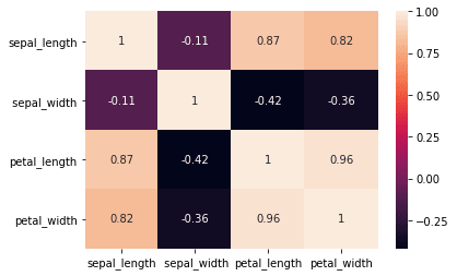
Another interesting case of data visualization is use a heatmap to visualize the correlation matrix of the dataset.

sns.heatmap(df.corr(), annot=True)

3. Preprocess the data

Frequently, the dataset collected from databases, files or scraping the internet is not ready to be consumed by a machine learning algorithm. In most cases, the dataset needs some kind of preparation or preprocessing before being used as input to a machine learning algorithm. In this case, we convert the string values of the class column to integer numbers because the algorithm we are going to use does not process string values.

df['class_encod'] = df['class'].apply(lambda x: 0 if x == 'Iris-setosa' else 1 if x == 'Iris-versicolor' else 2)
df['class_encod'].unique()

4. Select an algorithm and train the model

After exploring and preprocessing our data we can build our machine learning model to classify Iris specimens. So, the first step is to split our dataframe in input attributes and target attributes.

y = df[['class_encod']] # target attributes 
X = df.iloc[:, 0:4] # input attributes
X.head()

If in the previous step we splitted the dataframe by separating columns, in this step we split the data by rows. The method train_test_split() will split the X and y dataframes in training data and test data.

X_train, X_test, y_train, y_test = train_test_split(X, y, test_size=0.3,
                                                    random_state=0, stratify=y)

np.shape(y_train)

Then we use the datasets X_train and y_train to build a KNN classifier, using the KNeighborsClassifier class provided by scikit-learn. Because the machine learning algorithm is already implemented by the library, all we have to do is call the method fit() passing the X_train and y_train datasets as arguments.

m = KNeighborsClassifier()
m.fit(X_train, np.ravel(y_train))

Once the model is built, we can use the predict() method to calculate the predicted category of an instance. In this case, we want to predict the class of the first 10 lines of the X_test dataset. The return is an array containing the estimated categories.

m.predict(X_test.iloc[0:10])

We can use methods like score() and confusion_matrix() to measure the performance of our model. We see that the accuracy of our model is 1.0 (100%), which means that the model predicted correctly all cases of the test dataset.

m.score(X_test, y_test)
confusion_matrix(y_test, m.predict(X_test))

5. Save the model for later use

Finally, we want to save our model for later use. For example, we could embed our model into a webservice or mobile application. So we use the method dump() from the joblib package to save the model to a file.

dump(m, 'iris-classifier.dmp')

ic = load('iris-classifier.dmp')
confusion_matrix(y_test, ic.predict(X_test))

Conclusion

Although the simplicity of the Iris dataset, the steps demonstrated in this tutorial can be reproduced for practically any other dataset. The effort required on each step may vary, but the process is basically the same, so you can start practicing with simpler datasets and increase the complexity of your projects incrementally.

So, click the link below to open a ready to use template in Google Colab and create your first machine learning model right now:

First Machine Learning Model Template

Also, you can find a notebook version of this tutorial in the following link:

Iris Classification Tutorial