Prerequisites

Basic knowledge about graphs, linear algebra, and convolutional neural networks.

Introduction

In the field of Deep Learning (DL), particularly in Computer Vision (CV), Convolutional Neural Network (CNN) plays a vital part in extracting features of a given image. Structurally, images form a regular grid of integer values (0-255) divided into three channels (RGB). Therefore, one may visualize an image as a regular graph with nodes as the R, G, or B color value. For each non-edge pixel/node, there are eight edges to adjacent pixels/nodes. Taking advantage of this fixed structure, CNNs use 2D filters to perform the convolution operations.

However, various data sources are essentially graphs but do not follow a regular structure as that of images. For example, knowledge graphs, social networks, or even 3D meshes with vertices as the nodes. So how do we use deep learning magic on these data? This blog answers the question by:

1. Introducing the structure of a Graph Convolutional Networks(GCN).
2. Looking into the three underlying principles of convolutional operations in CNNs and GCNs.
3. Finally, understanding the forward propagation rule of GCNs.

1. Structure of a Graph Convolutional Networks(GCN).

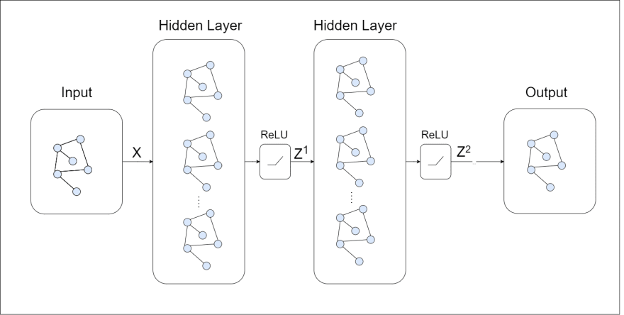
Structurally the following components form the GCN:

1. Input $(X)$ is a graph (represented as $G=(V, E)$ ), where $V$ denotes vertices and $E$ denotes edges) in the form of adjacency list $A$ and a feature matrix $X$ having the shape $N\times D$ ( $N$ is the number of nodes/vertices and $D$ is the number of input features).
2. Hidden Layers $(H)$ maintain the same graph structure. Also, their feature matrix $Z$ is of the shape $N\times F$ where $F$ is the number of features of a node for that layer.
3. Output $(Y)$ depends on the task at hand. For the semantic segmenting of a 3D mesh, it will be the same graph with the output matrix $Y$ of the shape $N\times C$ where $C$ is the number of classes. If we want to classify the entire graph, we will have to add a linear layer at the end of the last hidden layer to get the prediction.

As evident from the output of the GCN is a function that maps an input graph to the output by learning features of the graph.

2. The Three Underlying Principles of Convolution Operations.

In this section, we will compare the graph convolution (GC) layer with the basic convolution layer. Upon comparison, we will observe that a GC layer follows the same three principles as that of the convolution layer. After gaining this intuition, we will formulate the forward propagation rule for a GC layer in the following section.

So what are the three principles on which CNNs work and how are emulated in GCNs?

1. Locality: It states that during the convolution operation at a given position, the neighboring positions' values contribute towards determining its new value. For example, if we choose a 3 $\times$ 3 kernel, all the eight adjacent pixels contribute their values. Message passing in GCN allows it to follow the principle of locality. In fig. 2, the yellow nodes denote the locality of the green node.
2. Aggregation: This principle states that the local contribution of each node must be "summed-up," "meaned-over," or aggregated to get the new value. In the conventional convolution operation, it is the multiplication of adjacent pixels with the kernel weights. For graph convolution, it is the mean of the sum of values of the entire locality.
3. Composition: Standard convolution layers use the concept of composition (function-of-function) to increase their "field of perception." At a given instance, locality and aggregation serve to capture local features but doing this in composition allows information to pass over the area of a single convolution kernel. Consider fig. 2 again. At, $H^{l-1}$ while the green node was evaluating its new value based on adjacent nodes, so were the yellow nodes, as the kernel slid over them (for the standard convolution case). Therefore, at $H^{l}$ , all yellow nodes hold information of the red nodes also. As we calculate the new value for the green node at $H^{l}$ , we implicitly feed in the data of the non-adjacent red nodes; this is the true essence of message passing. For convolution layers, it is easy to observe that as we increase the size of the convolution filter, the "field of perception" increases proportionally with each step. With an expanded perception field - the networks capture more complex patterns in the data. As far as vanilla GCNs go, each composition allows the passing over of information from a node adjacent to the already established perception boundary.

3. The Forward Propagation Rule.

In this section, we will finally formulate the forward propagation rule for a graph convolution layer. Let's approach this by iteratively unveiling the equation.

As you can see, we have seven blanks to fill. Let's get going!

The first blank is quite simple. It's just the denotation of the $(l+1)^{th}$ GCN layer.

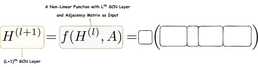
Now, we see that the $(l+1)^{th}$ GCN layer is a non-linear function having the inputs: the current GCN layer matrix and the adjacency matrix.

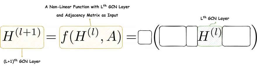
Finally, we move on to the actual function. The $l^{th}$ layer matrix is in between two other matrices yet to be revealed. Keep note that the shape of the $l^{th}$ layer matrix is $D\times F^{(l-1)}$ , where $D$ is the number of nodes, and $F^{(l)}$ is the number of features in the $l^{th}$ layer.

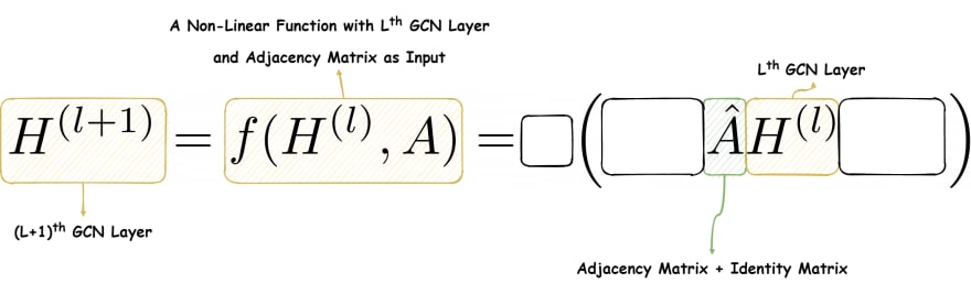
Moving on, we see that the $\hat{A}\ (A + I)$ matrix is in multiplication with $H^{(l)}$ . The first point of note: using $\hat{A}$ ensures that only the adjacent nodes and itself are selected during the multiplication. Thus, the locality principle is maintained. Further, the summation of their activations follows the aggregation principle. Secondly, we use $A + I$ instead of only $A$ because we want to enforce self-loops. That is, the current node's information must contribute to future calculation.

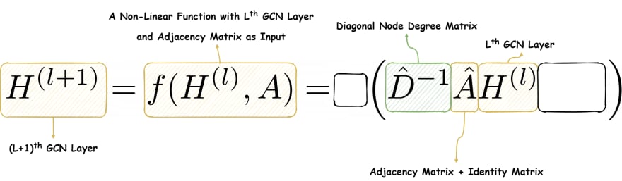
Summation of all the adjacent activations in a dense graph leads to an explosion of gradients, hence, the network becomes difficult to train. To mitigate this, we multiply the diagonal degree matrix of Ahat to average out the summed-up activations. In the end, $D^{-1}\hat{A}H$ produces an $N\times F^{(l-1)}$ matrix that has the normalized aggregated information from the locality.

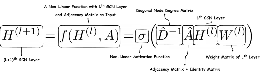
Now, this matrix is multiplied by the layer's weight matrix of the shape $F^{(l-1)}\times F^{(l)}.$ The weight matrix is trainable.

Finally, we get the activations of the layer by passing the $N\times F^{(l)}$ matrix through a non-linear activation function like ReLU. Basically, the network has converted a graph with nodes having features of dimension $F^{(l-1)}$ to $F^{(l)}$ .

The final equation in all it's glory is as follows:

A final note of interest is that we technically do not take the mean of the adjacent node values; instead, we use spectral normalization as mentioned in Kipf et. al. [2].

The modified equation is as follows:

Conclusion.

With this post, we delved deep into the theoretical foundation of a Graph Convolutional Network. The next post will show how powerful this simple setup is by semantically segmenting 3D meshes from the COSEG dataset. We will also look into how well these networks learn in a semi-supervised situation, that is when only a few labels are available per class. Stay tuned!

References.

[1] Kipf, T., 2016. How Powerful Are Graph Convolutional Networks?. [online] Tkipf.github.io. Available at: https://tkipf.github.io/graph-convolutional-networks/ [Accessed 20 October 2020].
[2] Kipf, T., & Welling, M. (2017). Semi-Supervised Classification with Graph Convolutional Networks. Retrieved 20 October 2020, from https://arxiv.org/pdf/1609.02907.pdf
[3] Published in Grandjean, Martin (2014). "La connaissance est un réseau". Les Cahiers du Numérique. 10 (3): 37–54. doi:10.3166/lcn.10.3.37-54. Retrieved 20 October 2020. [Banner credits]