
In this tutorial, we're going to walk through an example Machine Learning project where the goal is to predict the sale price of bulldozers.
This kind of problem is known as a regression problem because we're trying to determine a price, which is a continuous variable.
The data is from the Kaggle Bluebook for Bulldozers competition. We'll also use the same evaluation metric, root mean square log error, or RMSLE.
This exercise is a milestone project from the course Complete Machine Learning & Data Science Bootcamp, which I completed in March 2022.
You can find the Jupyter notebook in my GitHub repo.
The Workflow
Let's consider how we're approaching this problem, and the different steps to solve it.
We have a dataset provided to us. We'll approach the problem with the following 6-step machine learning modelling framework.

We'll use pandas, Matplotlib, and NumPy for data anaylsis. And we'll use Scikit-Learn for machine learning and modelling tasks.

After working through each step of this workflow, we'll have a trained machine learning model. And ideally, this trained model will be able to accurately predict the sale price of a bulldozer given different characteristics about it.
1. Problem Definition
The question that we're trying to answer is:
Given the characteristics of a particular bulldozer and data related to past sales of similar bulldozers, how well can we predict the future sale price of this bulldozer?
2. Data
Let's have a look at the dataset from Kaggle. First, we can see that it's a time series problem. That means the dataset contains a time attribute.
In this case, we're working with historical sales data for bulldozers. The dataset includes attributes such as model type, size, sale date, and more.
The 3 datasets available are:
-
Train.csv - Historical bulldozer sales data up to 2011 (with close to 400,000 examples with 50+ different attributes, including
SalePricewhich is the target variable). -
Valid.csv - Historical bulldozer sales data from January 1st, 2012 to April 30th, 2012 (close to 12,000 examples with the same attributes as
Train.csv). -
Test.csv - Historical bulldozer sales data from May 1st, 2012 to November 30th, 2012 (close to 12,000 examples, but missing the
SalePriceattribute, as this is what we aim to predict).
3. Evaluation
For this competition, Kaggle has set the evaluation metric to the root mean squared log error (RMSLE). The goal will be to get this value as low as possible.
To check how well our model is doing, we'll calculate the RMSLE and then compare our results to the Kaggle leaderboard.
4. Features
Features are the different parts of the data. During this step, we want to fin out what we can about the data and become more familiar with it.
A common way to do this is to create a data dictionary.
For this dataset, Kaggle provides a data dictionary containing information about what each attribute of the dataset means. We can download this file directly from the Kaggle competition page (account required) or view it on Google Sheets.
First, we'll import the dataset and start exploring it. And since we know the evaluation metric we're trying to minimise (RMSLE), our first goal is to build a baseline model and see how it compares against the competition.
Importing the data and preparing it for modeling
# Import data analysis tools
import pandas as pd
import numpy as np
import matplotlib.pyplot as plt
I've downloaded the data from Kaggle and stored it under the file path "./data/".
# Import the training and validation set
df = pd.read_csv("./data/bluebook-for-bulldozers/TrainAndValid.csv",
                 low_memory=False)
We can now start exploring our dataset with df.info(). Let's use matplotlib to visualize some of the data .
fig, ax = plt.subplots()
ax.scatter(df["saledate"][:1000], df["SalePrice"][:1000]);

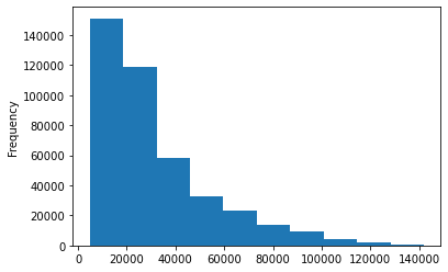
df.SalePrice.plot.hist();
Parsing dates
When working with time series data, it's a good practice to make sure dates are in the format of a datetime object (a Python data type which encodes specific information about dates).
df = pd.read_csv("./data/bluebook-for-bulldozers/TrainAndValid.csv",
                 low_memory=False,
                 parse_dates=["saledate"])
Now with parse_dates, we can see when calling df.info() that the dtype of "saledate" is datetime64[ns].
fig, ax = plt.subplots()
ax.scatter(df["saledate"][:1000], df["SalePrice"][:1000]);

To visualize the attributes of the DataFrame more easily, a trick is to transpose it with df.head().T.
Sort DataFrame by saledate
It makes sense to sort our data by date because we're working on a time series problem where we predict future values given past examples.
# Sort DataFrame by date (in ascending order)
df.sort_values(by=["saledate"], inplace=True, ascending=True)
df.saledate.head(5)
205615   1989-01-17
274835   1989-01-31
141296   1989-01-31
212552   1989-01-31
62755    1989-01-31
Name: saledate, dtype: datetime64[ns]
Make a copy of the original DataFrame
Since we're going to manipulate the data, it's better to make a copy of the original DataFrame and perform our changes there. This way, we keep the original DataFrame intact in case we need it again.
# Make a copy of the original DataFrame
df_tmp = df.copy()
Add datetime parameters for saledate column
We're doing this to enrich our dataset with as much information as possible.
Since we imported the data using read_csv() and parsed the dates using parase_dates=["saledate"], we can now access the different datetime attributes of the saledate column.
# Add datetime parameters for saledate
df_tmp["saleYear"] = df_tmp.saledate.dt.year
df_tmp["saleMonth"] = df_tmp.saledate.dt.month
df_tmp["saleDay"] = df_tmp.saledate.dt.day
df_tmp["saleDayofweek"] = df_tmp.saledate.dt.dayofweek
df_tmp["saleDayofyear"] = df_tmp.saledate.dt.dayofyear

# Drop original saledate
df_tmp.drop("saledate", axis=1, inplace=True)
5. Modeling
We've explored our dataset and enriched it with some datetime attributes. We could spend more time doing exploratory data analysis (EDA), finding more out about the data ourselves. But instead, we'll use a machine learning model to help us do EDA.
After all, one of the objectives when starting a new machine learning project is to reduce the time between experiments. So, let's move on to the model.
Following the Scikit-Learn machine learning map, we find that a RandomForestRegressor() is a good candidate.
from sklearn.ensemble import RandomForestRegressor
However, fitting the RandomForestRegressor() model with our training data would'nt work yet, because we've got missing numbers as well as attributes in a non-numerical format.
# Check for missing categories and different datatypes
df_tmp.info()
We see many columns have a type object.
# Check for missing values
df_tmp.isna().sum()
Likewise, many columns have missing values.
Convert strings to categories
One way to turn our data into numbers is to convert the columns with the string datatype into a category datatype.
To do this, we can use the pandas types API which allows us to interact and manipulate the types of data.
# These columns contain strings
for label, content in df_tmp.items():
    if pd.api.types.is_string_dtype(content):
        print(label)
This gives us a list of all the columns for which the data is in a string format.
# This will turn all of the string values into category values
for label, content in df_tmp.items():
    if pd.api.types.is_string_dtype(content):
        df_tmp[label] = content.astype("category").cat.as_ordered()
Calling df_tmp.info(), we see that the type object has been converted to category.
All of our data is now categorical. That means we can now turn the categories into numbers. However, we still have to deal with missing values.
In the format it's in, the data is good to be worked with, so let's save it to a file and reimport it so we can continue on.
Save processed data
# Save preprocessed data
df_tmp.to_csv("./data/bluebook-for-bulldozers/train_tmp.csv",
              index=False)

# Import preprocessed data
df_tmp = pd.read_csv("./data/bluebook-for-bulldozers/train_tmp.csv",
                     low_memory=False)
Our preprocessed DataFrame has the columns we added to it, but it's still missing some values. We can see where values are missing with df_tmp.isna().sum().
Fill missing values
Here are two things to know about machine learning models:
- All of our data has to be numerical
- There can't be any missing values
And as we've seen using df_tmp.isna().sum() our data still has plenty of missing values.
Filling numerical value
First, we're going to fill any column with missing values with the median of that column.
for label, content in df_tmp.items():
    if pd.api.types.is_numeric_dtype(content):
        print(label)
SalesID
SalePrice
MachineID
ModelID
datasource
auctioneerID
YearMade
MachineHoursCurrentMeter
saleYear
saleMonth
saleDay
saleDayofweek
saleDayofyear
# Check for which numeric columns have null values
for label, content in df_tmp.items():
    if pd.api.types.is_numeric_dtype(content):
        if pd.isnull(content).sum():
            print(label)
auctioneerID
MachineHoursCurrentMeter
# Fill numeric rows with the median
for label, content in df_tmp.items():
    if pd.api.types.is_numeric_dtype(content):
        if pd.isnull(content).sum():
            # Add a binary column which tells if the data was missing our not
            df_tmp[label+"_is_missing"] = pd.isnull(content)
            # Fill missing numeric values with median since it's more robust than the mean
            df_tmp[label] = content.fillna(content.median())
We can easily fill all of the missing numeric values in our dataset with the median. However, a value may be missing for a good reason. That's why we added a binary column which indicates whether the value was missing or not. This step helps to retain this information.
# Check if there's any null values
for label, content in df_tmp.items():
    if pd.api.types.is_numeric_dtype(content):
        if pd.isnull(content).sum():
            print(label)
Good, we no longer have any missing values.
Filling and turning categorical variables to numbers
Now, let's fill the categorical values. At the same time, we'll turn them into numbers.
# Turn categorical variables into numbers
for label, content in df_tmp.items():
    # Check columns which *aren't* numeric
    if not pd.api.types.is_numeric_dtype(content):
        # Add binary column to inidicate whether sample had missing value
        df_tmp[label+"_is_missing"] = pd.isnull(content)
        # We add the +1 because pandas encodes missing categories as -1
        df_tmp[label] = pd.Categorical(content).codes+1
All of our data is now numeric, and there are no missing values.
We should be able to build a machine learning model! Let's instantiate our RandomForestRegressor.
This will take a few minutes, which is too long for interacting with it. So, what we'll do is create a subset of rows to work with.
Splitting data into training and validation sets
According to the Kaggle data page, the validation set and test set are split according to dates. This makes sense since we're working on a time series problem.
Knowing this, randomly splitting our data into train and test sets using something like train_test_split() wouldn't work.
Instead, we'll split our data into training, validation, and test sets according to the date of the sample.
In our case:
- Training = all samples up until 2011
- Valid = all samples form January 1, 2012 - April 30, 2012
- Test = all samples from May 1, 2012 - November 2012
For more on making good training, validati, and test sets, check out the post How (and why) to create a good validation set by Rachel Thomas.
# Split data into training and validation sets
df_train = df_tmp[df_tmp.saleYear != 2012]
df_val = df_tmp[df_tmp.saleYear == 2012]

len(df_train), len(df_val)
(401125, 11573)
# Split data into X & y
X_train, y_train = df_train.drop("SalePrice", axis=1), df_train.SalePrice
X_valid, y_valid = df_val.drop("SalePrice", axis=1), df_val.SalePrice

X_train.shape, y_train.shape, X_valid.shape, y_valid.shape
((401125, 102), (401125,), (11573, 102), (11573,))
Building an evaluation function
The evaluation function they use for this Kaggle competition is the root mean squared log error (RMSLE).
It's important to understand the evaluation metric we're going for. The RMSLE is the metric of choice when we care more about the consequences of being off by 10% than being off by $10. That is, when we care more about ratios than differences. The MAE (mean absolute error) is more about exact differences.
Since Scikit-Learn doesn't have a built-in function for RMSLE, we'll create our own.
We can do this by taking the square root of Scikit-Learn's mean_squared_log_error (MSLE). MSLE is the same as taking the log of mean squared error (MSE).
While we're at it, we'll also calculate the MAE and R^2.
# Create evaluation function (the competition uses Root Mean Square Log Error)
from sklearn.metrics import mean_squared_log_error, mean_absolute_error

def rmsle(y_test, y_preds):
    return np.sqrt(mean_squared_log_error(y_test, y_preds))

# Create function to evaluate our model
def show_scores(model):
    train_preds = model.predict(X_train)
    val_preds = model.predict(X_valid)
    scores = {"Training MAE": mean_absolute_error(y_train, train_preds),
              "Valid MAE": mean_absolute_error(y_valid, val_preds),
              "Training RMSLE": rmsle(y_train, train_preds),
              "Valid RMSLE": rmsle(y_valid, val_preds),
              "Training R^2": model.score(X_train, y_train),
              "Valid R^2": model.score(X_valid, y_valid)}
    return scores
Testing our model on a subset of data
Traing an entire model would take far too long to continue experimenting as fast as we want to.
So, what we'll do is take a sample of the training set and tune the hyperparameters on that subset before training a larger model.
If our experiments are taking longer than 10-seconds, we should try to speed things up, by sampling less data or using a faster computer.
len(X_train)
401125
Let's alter the number of samples each n_estimator in the RandomForestRegressor sees using the max_samples parameter.
# Change max samples in RandomForestRegressor
model = RandomForestRegressor(n_jobs=-1,
                              max_samples=10000)
Setting max_samples to 10,000 means every n_estimator (by default 100) in our RandomForestRegressor will only see 10,000 random samples from our DataFrame, instead of the entire 400,000.
In other words, we'll be looking at 40x less samples, which means we'll get faster computation speeds. Though, we should expect our results to worsen (because the model has less samples to learn patterns from).
%%time
# Cutting down the max number of samples each tree can see improves training time
model.fit(X_train, y_train)
CPU times: user 43.5 s, sys: 1.39 s, total: 44.9 s
Wall time: 9.3 s
RandomForestRegressor(max_samples=10000, n_jobs=-1)
show_scores(model)
{'Training MAE': 5557.476079825491,
 'Valid MAE': 7145.432947377517,
 'Training RMSLE': 0.2576354132701014,
 'Valid RMSLE': 0.2932065424618794,
 'Training R^2': 0.860725458431776,
 'Valid R^2': 0.8334321554498396}
Hyperparameter tuning with RandomizedSearchCV
We can increase n_iter to try more combinations of hyperparameters but, in our case, we'll try 20 and see where it gets us. We're trying to reduce the amount of time between experiments.
%%time
from sklearn.model_selection import RandomizedSearchCV

# Different RandomForestClassifier hyperparameters
rf_grid = {"n_estimators": np.arange(10, 100, 10),
           "max_depth": [None, 3, 5, 10],
           "min_samples_split": np.arange(2, 20, 2),
           "min_samples_leaf": np.arange(1, 20, 2),
           "max_features": [0.5, 1, "sqrt", "auto"],
           "max_samples": [10000]}

rs_model = RandomizedSearchCV(RandomForestRegressor(),
                              param_distributions=rf_grid,
                              n_iter=20,
                              cv=5,
                              verbose=True)

rs_model.fit(X_train, y_train)
Fitting 5 folds for each of 20 candidates, totalling 100 fits
CPU times: user 9min 43s, sys: 38.7 s, total: 10min 22s
Wall time: 10min 30s
RandomizedSearchCV(cv=5, estimator=RandomForestRegressor(), n_iter=20,
                   param_distributions={'max_depth': [None, 3, 5, 10],
                                        'max_features': [0.5, 1, 'sqrt',
                                                         'auto'],
                                        'max_samples': [10000],
                                        'min_samples_leaf': array([ 1,  3,  5,  7,  9, 11, 13, 15, 17, 19]),
                                        'min_samples_split': array([ 2,  4,  6,  8, 10, 12, 14, 16, 18]),
                                        'n_estimators': array([10, 20, 30, 40, 50, 60, 70, 80, 90])},
                   verbose=True)
# Find the best parameters from the RandomizedSearch
rs_model.best_params_
{'n_estimators': 60,
 'min_samples_split': 6,
 'min_samples_leaf': 1,
 'max_samples': 10000,
 'max_features': 'auto',
 'max_depth': None}
# Evaluate the RandomizedSearch model
show_scores(rs_model)
{'Training MAE': 5623.00659389663,
 'Valid MAE': 7221.500628014852,
 'Training RMSLE': 0.2600757896526271,
 'Valid RMSLE': 0.2938688696407002,
 'Training R^2': 0.857223776894714,
 'Valid R^2': 0.8302372473994826}
Train a model with the best parameters
The course instructor, Daniel Bourke, tried 100 different combinations of hyperparameters (setting n_iter to 100 in RandomizedSearchCV) and found that the best results came from the ones we'll use below.
Note: This kind of search with n_iter = 100 can take about 2 hours on a powerful laptop. The search above with n_iter = 10 took only 10 minutes on my MacBook Air.
We'll instantiate a new model with these discovered hyperparameters and reset the max_samples back to its original value.
%%time
# Most ideal hyperparameters
ideal_model = RandomForestRegressor(n_estimators=90,
                                    min_samples_leaf=1,
                                    min_samples_split=14,
                                    max_features=0.5,
                                    n_jobs=-1,
                                    max_samples=None)
ideal_model.fit(X_train, y_train)
CPU times: user 10min 54s, sys: 5.69 s, total: 11min
Wall time: 1min 39s
RandomForestRegressor(max_features=0.5, min_samples_split=14, n_estimators=90,
                      n_jobs=-1)
show_scores(ideal_model)
{'Training MAE': 2927.714226014933,
 'Valid MAE': 5893.170337485774,
 'Training RMSLE': 0.14329949046791518,
 'Valid RMSLE': 0.2436971060471662,
 'Training R^2': 0.9596781605243438,
 'Valid R^2': 0.884359696206594}
With these hyperparameters and when using all the samples, we can see an improvement to our model's performance.
We could make a faster model by altering some of the hyperparameters. Particularly by lowering n_estimators since each increase in n_estimators is like building another small model.
However, lowering n_estimators or altering other hyperparameters may lead to poorer results.
Make predictions on test data
We've got a trained model so let's make predictions on the test data.
What we've done so far is training our model on data prior to 2011. However, the test data is from May 2012 to November 2012.
What we'll do is use the patterns that our model has learned on the training data to predict the sale price of a bulldozer with characteristics it has never seen before, but that are assumed to be similar to those found in the training data.
df_test = pd.read_csv("./data/bluebook-for-bulldozers/Test.csv",
                      parse_dates=["saledate"])
Unfortunately, the test data isn't in the same format as our other data, so we have to fix it. Let's create a function to preprocess our data.
Preprocessing the data
Our model has been trained on data formatted in a certain way. So, to make predictions on the test data, we need to take the same steps we used to preprocess the training data to preprocess the test data.
Note: Whatever we do to the training data, you have to do the same to the test data.
Let's create a function for doing so (by copying the preprocessing steps we used above).
def preprocess_data(df):
    # Add datetime parameters for saledate
    df["saleYear"] = df.saledate.dt.year
    df["saleMonth"] = df.saledate.dt.month
    df["saleDay"] = df.saledate.dt.day
    df["saleDayofweek"] = df.saledate.dt.dayofweek
    df["saleDayofyear"] = df.saledate.dt.dayofyear

    # Drop original saledate
    df.drop("saledate", axis=1, inplace=True)

    # Fill numeric rows with the median
    for label, content in df.items():
        if pd.api.types.is_numeric_dtype(content):
            if pd.isnull(content).sum():
                df[label+"_is_missing"] = pd.isnull(content)
                df[label] = content.fillna(content.median())

        # Turn categorical variables into numbers
        if not pd.api.types.is_numeric_dtype(content):
            df[label+"_is_missing"] = pd.isnull(content)
            # We add the +1 because pandas encodes missing categories as -1
            df[label] = pd.Categorical(content).codes+1

    return df
Note: This function could break if the test data has different missing values compared to the training data.
Now that we've got a function for preprocessing data, let's preprocess the test dataset into the same format as our training dataset.
We can see that our test dataset (after preprocessing) has 101 columns. But, our training dataset X_train has 102 columns (after preprocessing). Let's find the difference.
# We can find how the columns differ using sets
set(X_train.columns) - set(df_test.columns)
{'auctioneerID_is_missing'}
There wasn't any missing auctioneerID field in the test dataset.
To fix this, we'll add a column to the test dataset called auctioneerID_is_missing and fill it with False, since none of the auctioneerID fields are missing in the test dataset.
# Match test dataset columns to training dataset
df_test["auctioneerID_is_missing"] = False
Now the test dataset matches the training dataset and we should be able to make predictions on it using our trained model.
# Make predictions on the test dataset using the best model
test_preds = ideal_model.predict(df_test)
When looking at the Kaggle submission requirements, we see that to make a submission, the data must be in a certain format: a DataFrame containing the SalesID and the predicted SalePrice of the bulldozer.
# Create DataFrame compatible with Kaggle submission requirements
df_preds = pd.DataFrame()
df_preds["SalesID"] = df_test["SalesID"]
df_preds["SalePrice"] = test_preds
# Export to csv...
df_preds.to_csv("./data/bluebook-for-bulldozers/predictions.csv",
               index=False)
Feature Importance
By now, we've built a model which is able to make predictions. The people we share these predictions with might be curious to know what parts of the data led to these predictions.
This is where feature importance comes in. Feature importance seeks to find out which attributes of the data were the most important in predicting the target variable.
In our case, which bulldozer sale attributes had the most weight in the model to predict its overall sale price?
Beware: the default feature importances for random forests can lead to non-ideal results.
To figure out which features were most important in a machine learning model, a good idea is to search something like "[MODEL NAME] feature importance".
Doing this for our RandomForestRegressor leads us to find the feature_importances_ attribute.
Let's check it out.
# Find feature importance of our best model
ideal_model.feature_importances_

# Install Seaborn package in current environment (if you don't have it)
# import sys
# !conda install --yes --prefix {sys.prefix} seaborn

import seaborn as sns

# Helper function for plotting feature importance
def plot_features(columns, importances, n=20):
    df = (pd.DataFrame({"features": columns,
                        "feature_importance": importances})
          .sort_values("feature_importance", ascending=False)
          .reset_index(drop=True))

    sns.barplot(x="feature_importance",
                y="features",
                data=df[:n],
                orient="h")

plot_features(X_train.columns, ideal_model.feature_importances_);


Top comments (0)