
Linear regression is a basic predictive analytics technique that uses historical data to predict an output variable. It is popular for predictive modelling because it is easily understood and can be explained using plain English.
Linear regression models have many real-world applications in an array of industries such as economics (e.g. predicting growth), business (e.g. predicting product sales, employee performance), social science (e.g. predicting political leanings from gender or race), healthcare (e.g. predicting blood pressure levels from weight, disease onset from biological factors), and more.
Understanding how to implement linear regression models can unearth stories in data to solve important problems. We’ll use Python as it is a robust tool to handle, process, and model data. It has an array of packages for linear regression modelling.
The basic idea is that if we can fit a linear regression model to observed data, we can then use the model to predict any future values. For example, let’s assume that we have found from historical data that the price (P) of a house is linearly dependent upon its size (S) — in fact, we found that a house’s price is exactly 90 times its size. The equation will look like this:
P = 90*S
With this model, we can then predict the cost of any house. If we have a house that is 1,500 square feet, we can calculate its price to be:
P = 90*1500 = $135,000
In this blog post, we cover:
- The basic concepts and mathematics behind the model
- How to implement linear regression from scratch using simulated data
- How to implement linear regression using
statsmodels - How to implement linear regression using
scikit-learn
This brief tutorial is adapted from the Next XYZ Linear Regression with Python course, which includes an in-browser sandboxed environment, tasks to complete, and projects using public datasets.
Basic concepts and mathematics
There are two kinds of variables in a linear regression model:
- The input or predictor variable is the variable(s) that help predict the value of the output variable. It is commonly referred to as X.
- The output variable is the variable that we want to predict. It is commonly referred to as Y.
To estimate Y using linear regression, we assume the equation:
Yₑ = α + β X
where Yₑ is the estimated or predicted value of Y based on our linear equation.
Our goal is to find statistically significant values of the parameters α and βthat minimise the difference between Y and Yₑ.
If we are able to determine the optimum values of these two parameters, then we will have the line of best fit that we can use to predict the values of Y, given the value of X.
So, how do we estimate α and β? We can use a method called ordinary least squares.
Ordinary Least Squares
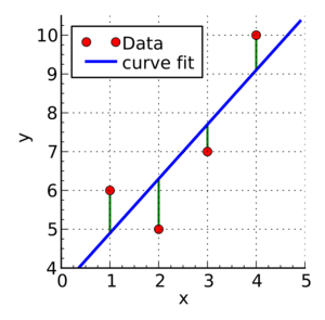
Green lines show the difference between actual values Y and estimate values Yₑ
The objective of the least squares method is to find values of α and β that minimise the sum of the squared difference between Y and Yₑ. We will not go through the derivation here, but using calculus we can show that the values of the unknown parameters are as follows:
where X̄ is the mean of X values and Ȳ is the mean of Y values.
If you are familiar with statistics, you may recognise β as simply
Cov(X, Y) / Var(X).
Linear Regression From Scratch
In this post, we’ll use two Python modules:
-
statsmodels— a module that provides classes and functions for the estimation of many different statistical models, as well as for conducting statistical tests, and statistical data exploration. -
scikit-learn— a module that provides simple and efficient tools for data mining and data analysis.
Before we dive in, it is useful to understand how to implement the model from scratch. Knowing how the packages work behind the scenes is important so you are not just blindly implementing the models.
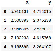
To get started, let’s simulate some data and look at how the predicted values (Yₑ) differ from the actual value (Y):
import pandas as pd
import numpy as np
from matplotlib import pyplot as plt

# Generate 'random' data
np.random.seed(0)
X = 2.5 * np.random.randn(100) + 1.5   # Array of 100 values with mean = 1.5, stddev = 2.5
res = 0.5 * np.random.randn(100)       # Generate 100 residual terms
y = 2 + 0.3 * X + res                  # Actual values of Y

# Create pandas dataframe to store our X and y values
df = pd.DataFrame(
    {'X': X,
     'y': y}
)

# Show the first five rows of our dataframe
df.head()
If the above code is run (e.g. in a Jupyter notebook), this would output something like:
To estimate y using the OLS method, we need to calculate xmean and ymean, the covariance of X and y (xycov), and the variance of X (xvar) before we can determine the values for alpha and beta.
# Calculate the mean of X and y
xmean = np.mean(X)
ymean = np.mean(y)

# Calculate the terms needed for the numator and denominator of beta
df['xycov'] = (df['X'] - xmean) * (df['y'] - ymean)
df['xvar'] = (df['X'] - xmean)**2

# Calculate beta and alpha
beta = df['xycov'].sum() / df['xvar'].sum()
alpha = ymean - (beta * xmean)
print(f'alpha = {alpha}')
print(f'beta = {beta}')
Out:
alpha = 2.0031670124623426
beta = 0.32293968670927636
Great, we now have an estimate for alpha and beta! Our model can be written as Yₑ = 2.003 + 0.323 X, and we can make predictions:
ypred = alpha + beta * X
Out:
array([3.91178282, 2.81064315, 3.27775989, 4.29675991, 3.99534802,
       1.69857201, 3.25462968, 2.36537842, 2.40424288, 2.81907292,
       ...
       2.16207195, 3.47451661, 2.65572718, 3.2760653 , 2.77528867,
       3.05802784, 2.49605373, 3.92939769, 2.59003892, 2.81212234])
Let’s plot our prediction ypred against the actual values of y, to get a better visual understanding of our model.
# Plot regression against actual data
plt.figure(figsize=(12, 6))
plt.plot(X, ypred)     # regression line
plt.plot(X, y, 'ro')   # scatter plot showing actual data
plt.title('Actual vs Predicted')
plt.xlabel('X')
plt.ylabel('y')

plt.show()

The blue line is our line of best fit, Yₑ = 2.003 + 0.323 X. We can see from this graph that there is a positive linear relationship between X and y. Using our model, we can predict y from any values of X!
For example, if we had a value X = 10, we can predict that:
Yₑ = 2.003 + 0.323 (10) = 5.233.
Linear Regression with statsmodels
Now that we have learned how to implement a linear regression model from scratch, we will discuss how to use the ols method in the statsmodelslibrary.
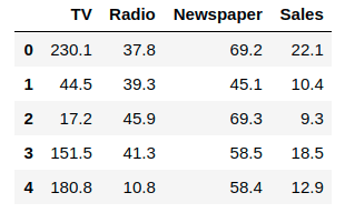
To demonstrate this method, we will be using a very popular advertisingdataset about various costs incurred on advertising by different mediums and the sales for a particular product. You can download this dataset here.
We will only be looking at the TV variable in this example — we will explore whether TV advertising spending can predict the number of sales for the product. Let’s start by importing this csv file as a pandas dataframe using read_csv():
# Import and display first five rows of advertising dataset
advert = pd.read_csv('advertising.csv')
advert.head()
First, we use statsmodels’ ols function to initialise our simple linear regression model. This takes the formula y ~ X, where X is the predictor variable (TV advertising costs) and y is the output variable (Sales). Then, we fit the model by calling the OLS object’s fit() method.
import statsmodels.formula.api as smf

# Initialise and fit linear regression model using `statsmodels`
model = smf.ols('Sales ~ TV', data=advert)
model = model.fit()
We no longer have to calculate alpha and beta ourselves as this method does it automatically for us! Calling model.params will show us the model’s parameters:
Out:
Intercept    7.032594
TV           0.047537
dtype: float64
In the notation that we have been using, α is the intercept and β is the slope i.e. α = 7.032 and β = 0.047.
Thus, the equation for the model will be: Sales = 7.032 + 0.047*TV
In plain English, this means that, on average, if we spent $100 on TV advertising, we should expect to sell 11.73 units.
Now that we’ve fit a simple regression model, we can try to predict the values of sales based on the equation we just derived using the .predict method.
We can also visualise our regression model by plotting sales_pred against the TV advertising costs to find the line of best fit:
# Predict values
sales_pred = model.predict()

# Plot regression against actual data
plt.figure(figsize=(12, 6))
plt.plot(advert['TV'], advert['Sales'], 'o')           # scatter plot showing actual data
plt.plot(advert['TV'], sales_pred, 'r', linewidth=2)   # regression line
plt.xlabel('TV Advertising Costs')
plt.ylabel('Sales')
plt.title('TV vs Sales')

plt.show()
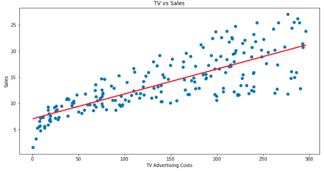
We can see that there is a positive linear relationship between TV advertising costs and Sales — in other words, spending more on TV advertising predicts a higher number of sales!
With this model, we can predict sales from any amount spent on TV advertising. For example, if we increase TV advertising costs to $400, we can predict that sales will increase to 26 units:
new_X = 400
model.predict({"TV": new_X})
Out:
0    26.04725
dtype: float64
Linear Regression with scikit-learn
We’ve learnt to implement linear regression models using statsmodels…now let’s learn to do it using scikit-learn!
For this model, we will continue to use the advertising dataset but this time we will use two predictor variables to create a multiple linear regression model. This is simply a linear regression model with more than one predictor, and is modelled by:
Yₑ = α + β₁X₁ + β₂X₂ + … + βpXp, where p is the number of predictors.
In our example, we will be predicting Sales using the variables TV and Radio i.e. our model can be written as:
Sales = α + β₁*TV + β₂*Radio.
First, we initialise our linear regression model, then fit the model to our predictors and output variables:
from sklearn.linear_model import LinearRegression

# Build linear regression model using TV and Radio as predictors
# Split data into predictors X and output Y
predictors = ['TV', 'Radio']
X = advert[predictors]
y = advert['Sales']

# Initialise and fit model
lm = LinearRegression()
model = lm.fit(X, y)
Again, there is no need to calculate the values for alpha and betas ourselves – we just have to call .intercept_ for alpha, and .coef_ for an array with our coefficients beta1 and beta2:
print(f'alpha = {model.intercept_}')
print(f'betas = {model.coef_}')
Out:
alpha = 2.921099912405138
betas = [0.04575482 0.18799423]
Therefore, our model can be written as:
Sales = 2.921 + 0.046*TV + 0.1880*Radio.
We can predict values by simply using .predict():
model.predict(X)
Out:
array([20.555464, 12.345362, 12.337017, 17.617115, 13.223908,
       12.512084, 11.718212, 12.105515,  3.709379, 12.551696,
       ...
       12.454977,  8.405926,  4.478859, 18.448760, 16.4631902,
        5.364512,  8.152375, 12.768048, 23.792922, 15.15754285])
Now that we’ve fit a multiple linear regression model to our data, we can predict sales from any combination of TV and Radio advertising costs! For example, if we wanted to know how many sales we would make if we invested $300 in TV advertising and $200 in Radio advertising…all we have to do is plug in the values!
new_X = [[300, 200]]
print(model.predict(new_X))
Out:
[54.24638977]
This means that if we spend $300 on TV advertising and $200 on Radio advertising, we should expect to see, on average, 54 units sold.
I hope you enjoyed this brief tutorial about the basics of linear regression!
We covered how to implement linear regression from scratch and by using statsmodels and scikit-learn in Python. In practice, you will have to know how to validate your model and measure efficacy, how to select significant variables for your model, how to handle categorical variables, and when and how to perform non-linear transformations.


Latest comments (7)
There is one thing I would have liked to see:
When you provided this formula/definition I would have liked to read something like this:
"It is called linear regression because it is linear in its parameters β"
or so. My ML/DL professor mentioned it on every of his slides about linear regression. Therefore an equation like
f(x) = ∑ βi x2
would be linear too, because it is linear in its parameters (β)
Beside that I really like your explanations! Definitely would like to read more about advanced topics :)
That's a great point. Thank you :) more coming soon!
As a beginner, i think your post is really clear. Nice work, keep going!
Thanks! Glad you liked it :)
Thank you so much for showing how to do it manually. There are so many articles showing different data analysis techniques, but a lot of them start off with:
This was sooooo nice to be able to sit through a nice, clear walkthrough of the math behind it with helpful graphs and visuals. It makes me so happy. Thanks again :)
I'm glad you enjoyed it! :) We'll be releasing a lot more tutorials in the upcoming months...is there anything in particular you'd like to learn?
Not specifically, but I would love to see more posts with more background on common data science algorithms and how they work.