
Photo by Matthew Ansley on Unsplash
In this tutorial, we'll create a Python package for computing image embeddings using a pretrained convolutional neural network (CNN) from the command line.
An image embedding is a numerical representation of an image that "embeds" it within a high-dimensional vector space. Image embeddings are useful for a variety of applications, including content-based information retreival and image classifiation. Furthermore, there are many off-the-shelf pretrained CNN architectures that you can use whenever you need. Machine learning engineers often use these pretrained models for benchmarks or as useful starting points.
After completing this tutorial, you will know how to:
- Load image data using
numpyandscikit-image - Compute linear image embeddings using PCA from
scikit-learn - Compute deep image embeddings using a pretrained ResNet model from Keras
- Remove any number of layers from a pretrained model in Keras
- Visualize deep image embeddings using UMAP
We are going to make a command line tool called embedding to do all of this. As a final demonstration, we will compare PCA with ResNet image embeddings of MNIST handwritten digits.
Setting up the embedding package
We're going to skip scaffolding out the embedding Python package and only walkthrough the development. First, you'll need to clone this repository:
git clone https://github.com/jmswaney/blog.git
cd blog/07_pretrained_image_embeddings
Within this folder, you'll see a pyproject.toml file as well as an environment.yml file for poetry and conda, respectively. You'll need to have conda installed on your system, and you can either follow my previous tutorial to install poetry globally or just use the one included in the embedding virtual environment. To install the virtual environment, you can run:
conda env create -f environment.yml
conda activate embedding
Note: I've included
cudatoolkitandcudnnin theenvironment.ymldependencies for GPU support. You can remove these dependencies if you don't want GPU acceleration.
Once installed and activated, we just need to install the Python dependencies, including the embedding CLI itself:
# from 07_pretrained_image_embeddings/
poetry install
This will install our machine learning dependencies like scikit-learn and tensorflow. It will also create an executable console script with its entrypoint connected to embedding:cli.
Developing the embedding CLI
The
embeddingfolder has the completed source code for this tutorial, so if you want to follow along with the development steps yourself, you may want to rename it and create an empty folder for your work.
Creating a simple entrypoint
The first thing we need to implement is a simple entrypoint function called cli and expose it from the package __init__.py. We can create cli.py and add a simple click command like in my CLI tutorial.
# in cli.py
import click

@click.command()
def cli():
    print("Hello, embedding!")
To expose this as embedding:cli, we just need to import it within our package's __init__.py.
# in __init__.py
__version__ = '0.1.0'

from .cli import *
Now we can check that our entrypoint is working from the terminal,
embedding
Hello, embedding!
By default, poetry installs the current package in "editable" mode, which means our source changes will take effect immediately in our CLI.
Loading image data
Next, we need to be able to load an image from a file. The best way I've found to do this is to use the imread function from scikit-image, which offers great speed and support for many lossless and lossy image formats. We can update the cli function to open an input image file.
import click
from skimage.io import imread

@click.command()
@click.argument("input")
def cli(input):
    print(main(input))

def main(input):
    return imread(input).shape
Testing this with a picture of a dog, it prints the shape of the image.
embedding data/dog.jpg
(333, 516, 3)
Now, we may also want to load data from Numpy arrays, so let's factor this out into a module specifically for I/O operations called io.py.
# in io.py
import os
import numpy as np
from skimage.io import imread

NUMPY_EXT = ".npy"

def load(filename: str) -> np.ndarray:
    ext = os.path.splitext(filename)[-1]
    if ext == NUMPY_EXT: return np.load(filename)
    return imread(filename)
Then loading .npy and .npz files should work as well,
embedding data/dog.npz
(333, 516, 3)

embedding data/dog.npy
(333, 516, 3)
Linear embeddings with PCA
Before we get to using pretrained image models, let's set the stage with principal component analysis (PCA). PCA is an unsupervised learning algorithm that will calculate a linear projection to a lower-dimensional space that preserves as much of the variance in the original dataset as possible.
We'll need multiple images for this, so let's randomly sample square patches from our example image. Then, in a new embed.py module, we can use sklearn to calculate our PCA embedding.
# in cli.py
from embedding.io import load
from embedding.embed import pca
import numpy as np
from random import random
from math import floor

def main(input):
    data = load(input)

    size = 64
    start = lambda: (floor(random()*(data.shape[0] - size)), floor(random()*(data.shape[1] - size)))
    x = np.asarray([data[y:y+size, x:x+size] for (y, x) in [start() for _ in range(32)]])
    print("Patches shape", x.shape)

    x_pca = pca(x.reshape(len(x), -1), 4)
    print("PCA embedded shape", x_pca.shape)
Since PCA applies to vector inputs, we needed to reshape our images into vectors. When we run this, we can see the data dimensionality is reduced, as expected.
embedding data/dog.jpg

Patches shape (32, 64, 64, 3)
PCA embedded shape (32, 4)
Here, we've sampled 32 image patches, each (64, 64, 3), and we have chosen to use 4 principal components.
Deep embeddings using ResNet50V2
Now that we have our PCA image embeddings working, we can move to a pretrained neural network. Keras has several CNNs available with weights obtained from ImageNet pretraining here. To keep things simple, we'll just use the ResNet50V2 achitecture for demonstration.
Within our embed.py module, we can import the model and instantiate it with the ImageNet weights. The first time we do this, Keras will download the weights and keep them locally cached. We need to make sure that we instantiate the model with include_top=False so that we get the last hidden representation in the network (as opposed to class label probabilities from the final softmax layer).
import numpy as np
from sklearn.decomposition import PCA
import tensorflow as tf
from tensorflow.keras.applications.resnet_v2 import preprocess_input

def pca(x: np.ndarray, n: int) -> np.ndarray:
    return PCA(n_components=n).fit_transform(x)

def resnet(x: np.ndarray) -> np.ndarray:
    model = tf.keras.applications.ResNet50V2(include_top=False)
    maps = model.predict(preprocess_input(x))
    if np.prod(maps.shape) == maps.shape[-1] * len(x):
        return np.squeeze(maps)
    else:
        return maps.mean(axis=1).mean(axis=1)
Notice that we also used the Keras utility function preprocess_input for the resnet_v2 family of models. This is important to make sure that we are scaling our images to intensity values between -1 and 1, as the model was trained on images that were scaled similarly. We also perform global average pooling to return a vector representation, effectively removing any remaining spatial information left in the activation maps.
When we call resnet with our image patches in cli.py, we get the following,
embedding data/dog.jpg

Patches shape (32, 64, 64, 3)
PCA embedded shape (32, 4)
ResNet embedded shape (32, 2048)
This shows that the ResNet50V2 architecture provides a 2048-dimensional embedding from the last layer of the model.
Note: if you encounter GPU memory allocation issues, then you may need to allow memory growth using this suggestion.
Saving image embeddings
Now that we can compute our image embeddings, we need a way for our CLI to save them to a file. Back in our io.py module, we can use numpy again to save our image embeddings with optional lossless compression.
# in io.py
def save(filename: str, x: np.ndarray, compress: bool) -> None:
    np.savez_compressed(filename, x) if compress else np.save(filename, x)
At this point, it would be helpful to refactor our main function into a slightly more scoped embed function that uses a given model to embed images as numpy arrays.
# in embed.py
def embed(x: np.ndarray, model: str, n: int):
    match model:
        case "pca":
            return pca(x.reshape(len(x), -1), n)
        case "resnet":
            if x.ndim == 3:
                return resnet(np.repeat(x[..., np.newaxis], 3, axis=-1))
            return resnet(x)
        case _:
            raise Exception("Invalid model provided")
We've repeated black and white images in the last dimension to match the expected input dimensionality for ResNet50V2.
We can use this in cli.py which uses io.py to perform side-effecting operations.
# in cli.py
MODEL_TYPES = ['pca', 'resnet']

@click.command()
@click.argument("input")
@click.argument("output")
@click.option("--model", "-m", required=True, type=click.Choice(MODEL_TYPES))
@click.option("--dimensions", "-d", "n_dim", default=32, type=int)
@click.option("--compress", "-c", is_flag=True)
def cli(input, output, model, n_dim, compress):
    x = sample_patches(load(input), 32, 64)
    x_embed = embed(x, model, n_dim)
    save(output, x_embed, compress)
We've added arguments to write the output file with optional compression as well as choose which model to use and the embedding dimension (for PCA). We've also refactored the image patch sampling code into the sample_patches function.
Loading MNIST data
Since it's uncommon to be embedding a single image, we can remove our sample_patches function. If the input is a numpy array, we assume it has the proper dimensionality for the downstream models. If the input is a folder, we should assume it is a flat folder of only images which should all be embedded in alphanumerical order. We'd also like the ability to load the MNIST training images. To perform all these loading operations, we can edit the load function in io.py,
from typing import Optional
import os
import numpy as np
from skimage.io import imread
from tensorflow.keras.datasets.mnist import load_data

MNIST_NAME = "mnist"
MNIST_CACHE = "mnist.npz"
NUMPY_EXT = ".npy"

def load(name: str) -> tuple[np.ndarray, Optional[np.ndarray]]:
    if name == MNIST_NAME:
        return load_data(MNIST_CACHE)[0] # Only training set
    ext = os.path.splitext(name)[-1]
    if ext == NUMPY_EXT: return np.load(name)
    return np.asarray([imread(os.path.join(name, x)) for x in os.listdir(name)])
So if we pass "mnist" as the first argument to embedding, we'll get the image data and labels from the MNIST dataset in Keras. Otherwise, we'll load the given matrix or folder of images.
Generating UMAP visualizations
We often want to visualize high-dimensional embeddings on a 2D plot. The most common tools for this are TSNE and UMAP, so for our example, we'll add an option to generate a UMAP plot of the image embeddings.
Back in our embed.py module, we'll add the following:
from umap import UMAP

def umap(x, seed = None):
    if seed: np.seed(seed)
    return UMAP().fit_transform(x)
We can call this in cli.py to save our results to a file.
from embedding.io import load, save
from embedding.embed import embed, umap
from embedding.plot import plot_umap, plot_pca
import os
import click

MODEL_TYPES = ['pca', 'resnet']

@click.command()
@click.argument("input")
@click.argument("output")
@click.option("--model", "-m", required=True, type=click.Choice(MODEL_TYPES))
@click.option("--dimensions", "-d", "n_dim", default=32, type=int)
@click.option("--compress", "-c", is_flag=True)
@click.option("--plot", "-p", is_flag=True)
@click.option("--seed", "-s", type=int, default=None)
def cli(input, output, model, n_dim, compress, plot, seed):
    x, y = load(input)
    print("Input shape", x.shape)
    x_embed = embed(x, model, n_dim)
    print("Embedded shape", x_embed.shape)
    save(output, x_embed, compress)
    if plot:
        root, ext = os.path.splitext(output)
        name = os.path.basename(root)
        if x_embed.shape[-1] == 2:
            plot_pca(x_embed, y, f"{name}_pca.png")
        else:
            x_umap = umap(x_embed, seed)
            print("UMAP shape", x_umap.shape)
            save(f"{name}_umap{ext}", x_umap, compress)
            plot_umap(x_umap, y, f"{name}_umap.png")
We added a _umap suffix to the output plot and matrix filenames for UMAP results (if the embedding dimension isn't already 2). If the embedding dimension is 2, then we just assume it's from PCA, and we plot it without performing UMAP.
We can write the plot_pca and plot_umap function in plot.py.
from typing import Optional
from matplotlib import pyplot as plt
import seaborn as sns
import numpy as np

sns.set(style="white", context="poster", rc={ "figure.figsize": (14, 10), "lines.markersize": 1 })

def make_scatter(x: np.ndarray, y: Optional[np.ndarray]):
    if y is None:
        plt.scatter(x[idx, 0], x[idx, 1])
    else:
        for label in np.unique(y):
            idx = np.where(y == label)[0]
            plt.scatter(x[idx, 0], x[idx, 1], label=label)
            plt.legend(bbox_to_anchor=(0, 1), loc="upper left", markerscale=6)

def plot_umap(x: np.ndarray, y: Optional[np.ndarray], filename: str):
    make_scatter(x, y)
    plt.xlabel("UMAP 1")
    plt.ylabel("UMAP 2")
    plt.title(filename)
    plt.savefig(filename)

def plot_pca(x: np.ndarray, y: Optional[np.ndarray], filename: str):
    make_scatter(x, y)
    plt.xlabel("PC 1")
    plt.ylabel("PC 2")
    plt.title(filename)
    plt.savefig(filename)
In make_scatter, we use seaborn and matplotlib to scatter plot all 2D image representations along with class labels if we have them.
Removing any number of layers
It's often helpful to remove more layers than just the top softmax layer, and this is an area that you can experiment with. Since convolutional architectures are typically structured in blocks, it's often worthwhile to remove entire blocks when trying to use pretrained models in a new image domain.
We can add a command-line argument to specify how many layers we'd like to keep (at which point in the original model do we stop and use as our image embedding). If this argument is not specified, then we take the enitre model without the top.
# Add option to cli.py
...
@click.option("--layers", "-l", type=int, default=None)
def cli(input, output, model, n_dim, layers, compress, plot, seed, batch_size):
    ...
    x_embed = embed(x, model, n_dim, batch_size, layers)
    ...

# Remove layers in embed.py
def resnet(x: np.ndarray, batch_size = None, layers = None) -> np.ndarray:
    full = tf.keras.applications.ResNet50V2(include_top=False)
    model = full if layers is None else tf.keras.models.Model(full.input, full.layers[layers].output)
    ...
Now if we pass --layers 100, we'll get the first 100 layers of the ResNet50V2 model.
Results
Now that we've completed the initial development of our embedding tool, it's time to use it. First, let's look at a simple 2D PCA image embedding.
# Embed MNIST using 2D PCA
embedding mnist mnist_pca_2d.npy --model pca -d 2 -p

The first principal component looks like it corresponds roughly to having a hole in the center of the digit (zero-like).
Now let's compare this to our ResNet50V2 image embedding visualized with UMAP.
# Embed MNIST using ResNet50V2
embedding mnist mnist_resnet.npy --model resnet -p -s 582

It seems that in both image embeddings, 0 and 1 are the most obvious digits to identify. While the ResNet image embeddings have 0 and 1 separated slightly better than the PCA plot, it's surprisingly not that much better. Perhaps we can use fewer layers on this simpler dataset.
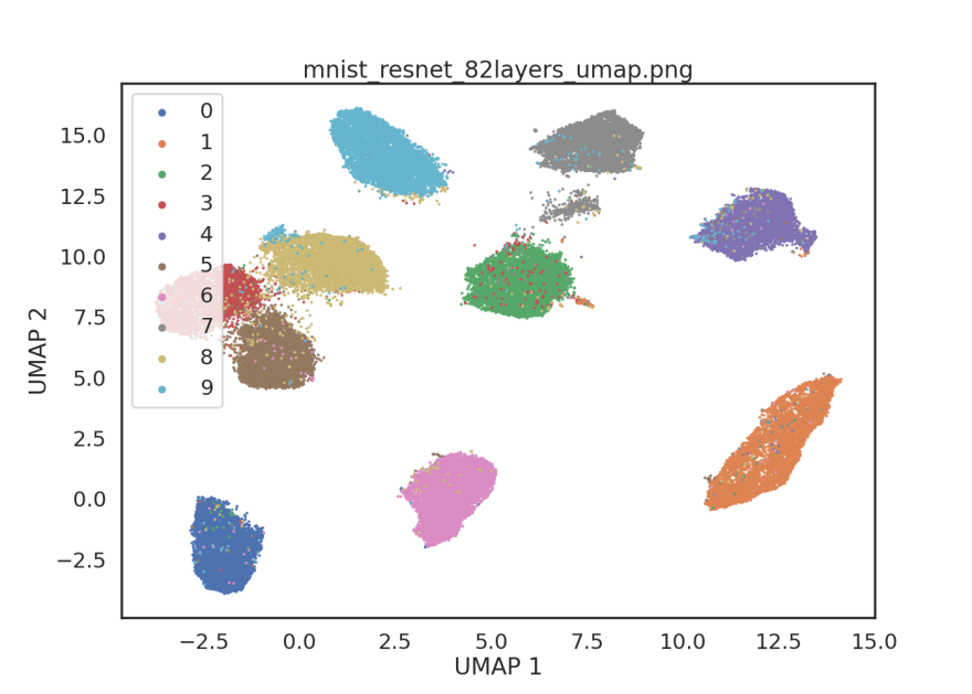
After some experimentation, I've found that removing blocks 4 and 5 from the ResNet50V2 model give image embeddings that are closer to linearly separable. Removing blocks 4 and 5 corresponds to taking the first 82 layers of the model.
# Embed MNIST using 82 layers of ResNet50V2
embedding mnist mnist_resnet_82layers.npy --model resnet -p -s 582 -l 82
Final thoughts
Making use of pretrained models is an essential tool in the toolbox for machine learning engineers. Pretrained image embeddings are often used as a benchmark or starting point when approaching new computer vision problems. Several architectures that have performed extremely well at ImageNet classification are avilable off-the-shelf with pretrained weights from Keras, Pytorch, Hugging Face, etc.
Here, we've created a simple Python package to help in the computation of image embeddings from the command-line. We used our embedding CLI to compute and visualize MNIST image embeddings using PCA and a ResNet50V2 model. In this relatively simple dataset, we found that using a subset of layers from the ResNet50V2 model performed qualitatively better than PCA at distinguishing between handwitten digits (without supervised training).
We might have expected the earlier layers of the ResNet50V2 model to be more applicable to the MNIST dataset because earlier layers in CNN's are known to extract features related to edges and textures. The higher-level visual features needed to classify the thousands of RGB natural images in ImageNet may not be as helpful when dealing with black and white images of handwritten digits.
Source availability
All source materials for this article are available here on my blog GitHub repo.


Oldest comments (0)