Congratulations - You have just landed a new job as a Data Scientist 😀! In your first month, you need to start analyzing tons of data. But before you start unlocking insights and predicting future trends, you need to access these data in order to explore it. Yikes! Did you wish you just started predicting future trends right away? Smiles, You are not Doctor Fate!

These tons of data can vary greatly in form and they are commonly seen in a tabular structure, where we have rows (also known as records, observations etc) and columns (also known as features, variables, fields etc) - like in 1.md below:

Data in .csv and .xlsx files have a tabular-like structure and in order to work efficiently with this kind of data in Python, we need to use the Pandas package. In Pandas, there is a data structure that can handle tabular-like structure of data - this data structure is called the DataFrame. Look at 2.md below to see the DataFrame version of the 1.md:

In 2.md, you can see a similar structure like in 1.md - we also have rows and columns - each row has a unique row label - NG, CA, BR, CH, FR. The columns also have labels - country, capital, population_millions. So, how do you put this data in a DataFrame to start exploring? Also for you to explore it well, what are the different ways to access the data in this DataFrame? Cheers! You are about to start your journey on becoming a Pandas Pundit!

You are given tons of data in a CSV file as seen below in 3.csv:

First of all, to get the data in 3.csv into a DataFrame, look at 4.py below:

which returns the DataFrame in 5.txt below:

Now that we have our data in a DataFrame, it is time to access it. There are several ways to access or select or index or subset or slice data in DataFrames - Data can be accessed via:

1. square brackets: [ ]
2. loc: label-based
3. iloc: position-based
4. at: label-based
5. iat: position-based

Let’s see how you can access data in columns only, rows only and both rows and columns from the Dataframe in 5.txt using the 5 ways above:

square brackets [ ] - 1

Let's look at column access and row access using []:
1.1: Column Access:
We have single column access and multiple column access.
1.1.1: single column access:
To access data in the Country column in 5.txt above, for example, we do:

which returns:

In 7.txt above, the dtype (datatype) of the what is returned is an object. The type of object returned can be known using:

In 8.py above, it is a pandas Series object. A pandas series is a 1D (1-Dimensional array) that can be labelled just like the DataFrame, a series has row labels/indexes. So, with this, it shows that a collection of series creates a DataFrame.

This series object returned can also be accessed using the square brackets. For example, to grab the value Nigeria in 7.txt above, see 9.py below:

Also, note that I can use the dot notation as seen in lines 19-20 above. Use the dot notation when the column name does not contain any special characters or spaces and is not a keyword in python.

However, if you want a DataFrame returned and not a series - use double square brackets as seen in 10.py below:

1.1.2: multiple column access:
To access more than one column in 5.txt, we do:

which returns:

1.2: Row Access:
The only way of accessing rows in a DataFrame using the square brackets way is by specifying a slice on the row. Specifying a slicing index takes the form - start:stop:step/stride

Indices are either numeric which is the default or labelled. Let's dive deeper below:

1.2.1: default numeric indices:
Given [x:y:z] as a slicing index, it means count in increments of z starting at x inclusive, up to y exclusive - for numeric indexes, the stop index is always exclusive.

Take a look at this figure below:

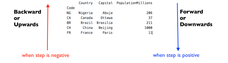
In the figure above, the direction in which my rows are returned is determined by the sign of the step/stride i.e z, given [x:y:z].

• If the step/stride is positive, start from the specified index position of the DataFrame and go the downward/forward direction when returning rows*.
• If it is negative, start from the specified index position of the DataFrame and move upwards/backwards when returning rows.

Given [:y:-z] as a slicing index, start from the last row in the DataFrame and go backwards/upwards but If [:y:z] is given, start from the first row in the DataFrame and go forward/downward.

In the forward/downward or in the backward/upward direction, the start index should always come before the stop index else no rows will be returned.

Let us take a look below at how positive and negative strides works:

1.2.1.1: positive step(s)/stride(s) :

In 13.py, lines 3-9 above, we use the default numeric index. It has this structure start:stop:[step or stride] - [step or stride] in square brackets means it is optional. Given countries[1:3], 1 is the start while 3 is the stop. When the step or stride is not specified like it is the case here, it has a default value of 1.

In 13.py, lines 11-18 above - given countries[2:] - note that the stop index is omitted i.e the explicit end index position is omitted. countries[2:] returns rows starting with the row with index position 2 till the last row in the DataFrame inclusive as seen above. : is a universal slice. If its left-endpoint (start) is omitted then the rows returned starts from the very first row in the DataFrame but if the right-endpoint is omitted, the row returned is till the very last row in the DataFrame inclusive.

In 13.py, lines 20-27 above - given countries[:3] - note that the start index is omitted i.e the explicit start index position is omitted.
countries[:3] returns rows starting with the first row till the row with index position 2 inclusive - remember that a numeric stop index is exclusive: so, the row at index position 3 is not returned as seen above.

In 13.py, lines 29-38 above, given countries[:] - note that both the start and stop indices are omitted i.e the explicit start and stop indices positions are omitted. countries[:] returns rows starting from the start of the row till the last row inclusive i.e it returns every row.

In 13.py, line 40-47 above, given countries[::2], using the formula above, this means counts in increment/steps/strides of 2 starting from the first row up to the last row inclusive i.e it returns every 2nd row. So, this is how it works - it return rows

• starting from the first row which has index 0,
• add steps of 2 i.e index 0 + 2 = index 2; then index 2 + 2 = index 4
• so, we have rows with index positions 0, 2, 4 returned

In 13.py, lines 49-54 above, given countries[-1:] - note the
following below -

• the DataFrame, countries, has rows labelled NG, CA, BR, CH, FR. These rows also have default numeric indices which can be positive 0, 1, 2, 3, 4 or negative -5, -4, -3, -2, -1.
• countries[-1:] is the same as countries[-1::1] - so we start from the last row and go downwards - downwards since the step/stride is positive
• this returns only the last row because there is no other row downwards

In 13.py, lines 56-64 above, given countries[:-1] - it returns rows
starting from the first row but excludes the last row.

In 13.py, lines 66-72 above, given countries[-2:] - it returns rows starting from the last but one row till the last row inclusive.

In 13.py, lines 74-81 above, given countries[:-2] - it returns rows
starting from the first row till it includes the row before last but one
row.

In 13.py, lines 83-88 above, given countries[-1:-1] - it returns
an empty DataFrame - starts from the last row but excludes the last
Row, hence nothing is returned.

1.2.1.2: negative step(s)/stride(s) :
With negative steps, rows get returned backwards. Let us see some examples in 14.py below:

In 14.py, lines 3-8 above, given countries[3:-4:-1] - note the following below:

• the stride/step is negative, so rows get returned backwards/upwards - when you look at the tabular-like structure in 5.txt above, we start getting rows from the end depending on the specified index and then go upwards/backwards i.e from the row with label CH and then move upwards.
• the stop has a negative value of -4 which is the row labelled CA. So, this row and the ones after it is not be included in the rows returned
• hence we have just two rows labelled CH and BR returned.

In 14.py, lines 11-17 above, given countries[4:-4:-2] - note the following below:

• the stride/step is negative and in steps of 2
• so we return rows starting from index position 4, then go upwards/backwards i.e from row with label FR and then move upwards/backwards but excludes row with index position 4 with all other rows after it too.

In 14.py, lines 19-24 above, given countries[0: -1: -1], it returns an
empty DataFrame. Here is why:

• Since the step/stride is negative we start at 0 and then go upwards or backwards - but it seems the stop index comes before the start index - so this cannot work, hence an empty DataFrame is returned

1.2.1: Labelled indexes:
With labelled indexes, it also takes the form start:stop:step/stride. But here are some things to take note of below:

• The stop label is inclusive, unlike numeric indices where the stop index is exclusive.
• Pairing labelled and numeric indices in the start or stop indices are not allowed e.g countries[‘NG’: 4] would give an error
• The step/stride is still numeric and can also be positive or negative
• and of course, all rules that go with having positive or negative step/stride applies here too.

Let’s see some examples in 15.py below:

In 15.py, lines 3-10 above, given countries[‘CA’:’CH’], we can see that the rows returned includes the row with the label CH which is the stop index label specified.

In 15.py, lines 12-20 above, given countries[:’CH’], the rows returned starts from the first row in the DataFrame till it includes the row labelled CH.

In 15.py, lines 22-30 above, given countries[‘CA’:], the rows returned starts from the row labelled ‘CA’ in the DataFrame till it includes the last row.

In 15.py, lines 32-39 above, given countries[‘NG’::2], the rows returned -

• starts from the row labelled ‘NG’ in the DataFrame
• add steps of 2 - index NG has a default index position of 0, so 0 + 2 = index 2 which is the row labelled BR; then index 2 + 2 = index 4, which is the row labelled FR
• so, we have rows labelled NG, BR, FR which have default numeric index positions 0, 2, 4 returned.

In 15.py, lines 41-49 above, given countries[:‘CA’:-1], the rows
returned -

• starts from the last row labelled FR in the dataframe
• add steps of -1 :
  • index FR has a default negative index position of -1, so -1 + -1 = index -2 which is the row labelled CH
  • then index -2 + (-1) = index -3, which is the row labelled BR
  • then index -3 + (-1) = index -4, which is the row labelled CA
• so, we have rows labelled FR, CH, BR, CA which have default numeric index positions -1, -2, -3, -4 returned.

Using square brackets, [ ] has its limitations like the ability to select several rows and columns at the same time. So, let's jump into loc and iloc to see its awesomeness!

loc - 2

2.1: Row Access:
By default, loc accesses rows. Loc is label-based, so I just need to specify the row label. Let us see some examples in 16.py below:

In 16.py, lines 3-16 above, given countries.loc[‘FR’] or countries.loc[[‘FR’]], the row with label FR returns a series or dataframe respectively.

In 16.py, lines 18-25 above, given countries.loc[[‘CA’, ‘BR’, ‘CH’]], the rows with labels listed in the square brackets are returned

2.2: Row and Column Access:
We can simultaneously access rows and columns using loc. It takes the form countries.loc[row, column]. Let us see some examples below in 17.py:

In 17.py, lines 3-10 above, given countries.loc[['CA', 'BR', 'CH'], ['Country',
'Capital']] - we specify a list of row labels and also a list of column labels we want to be returned.

In 17.py, lines 12-50 above, we can see slices can also be specified. Everything we have seen so far in relation to positive or negative steps/strides also applies here as seen in the examples given.

2.3: Column Access:
We can also select the specific columns we need while we select all rows as seen below in 18.py:

iloc - 3

Just like loc, iloc is row-based by default. The difference is that iloc is position-based. let's see some examples in 19.py below:

19.py above gives the iloc version of the examples given for loc for row access, row and column access and column access. As I earlier said, the only difference is that iloc is position-based while loc is label-based.

Kindly note that ix, which is also a way to accessing data in a DataFrame, is deprecated in favour of loc and iloc, so it is not advisable to use it the ix indexer.

at - 4

at is label-based like loc but it is used only to access a single value in a DataFrame. Unlike loc, which can not just get a single value but also several values as we have seen above.

See some examples below in 20.py:

iat - 5

iat is position-based like iloc but also accesses a single value like at. See some examples below in 21.py:

Now, let's summarize the key points together:

• Accessing data using indices takes the form, [start:stop:step]
• Numeric stop indices are exclusive
• Label stop indices are inclusive
• A step can be positive or negative - When it is positive, start at the specified index then go downwards/forward but when it is negative, start at the specified index then go upwards/backwards.
• Given [:y:-z] as a slicing index, start from the last row in the DataFrame and go backwards/upwards.
• Given [:y:z] is given, start from the first row in the DataFrame and go forward/downward*.
• loc - label-based
• iloc - position-based
• at - label-based but returns a single value
• iat - position-based but returns a single value

Wowww! That was so much to take in. But you are on your way in becoming a Pandas Pundit! Stay tuned on this series for my next article on Filtering Data in Dataframes! Have an amazing and fulfilled week ahead!