Title
- Very deep convolutional networks for large scale image recognition
- result:
-
Large Scale image recognition
-
- Method
Very deep convolution
Abstract
- Why / aim: To investigate the effect of the depth on accuracy of recognition
- Description / method: By increasing the depth using an architecture with very small (3*3) convolution filter increasing depth upto 16-19 weight layers
- Result: model that genralize well on other datasets as well
Introduction
- Background:
Convolution networks have seen great success in large scale image and video recognition
This is possible due to:
- Large public image datasets
- high performance systems
- large scale distributed clusters
- Intention:
This paper address an important aspect of ConvNet architecture design i.e.
depth. In this paper, authors keeps other aspects constant while steadily increasing depth of the network by adding 3*3 filter convolution layers
Data
-
Dataset
ILSVRC-2012 dataset
It includes 1000 classes which are divied as following:- Training
1.3 Million - Validation
50 Thousand - testing
100 Thousand
Perfomance Evalution is done in 2 ways
- Top - 1 / multi class classification error: the problem of classifying instances into one of three or more classes
- Top - 5: The proportion of images such that ground truth category is outside the top 5 predicted categories
- Training
-
Preprocessing:
- isotropically rescalling (i.e. keeping image ratio same while scalling) to 224
- subtracting mean RGB value
- Random cropping one crop per image per SGD iteration
- Random horizontal flips
- Random RGB shift
Model Architecture
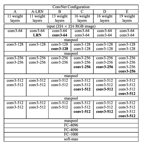
Input fixed size RGB image of 224*224 px.followed by preproccessing steps.
Architecture is stack of convolution layers with filters of smallreceptive field: 3*3 or 1*1 in some cases
1*1 convolution layers can be treated as linear transformation followed by non-linear transformation.
Stride is fixed to 1 px . Padding is such that size is maintained.
pooling is done by max pooling layers with 2*2 window and stride 2.
After this 3 FC layers are used.
2 have 4096 channels and last one is 1000 way soft-max layer.
All hidden layers used ReLU.
also, some models used Local response Normalization but it did not improve the performance while increasing memory consumption and computation time.
There are 6 (A-E, A-LRN) models based on this genaric design
A-E 5 models differ only in depth from 11 to 19 layers.
With width of convolution layers starting from 64 to 512 increasing in factor of 2.
Input and Output
- Input:
fixed size 224*224 RGB image - Output:
class
New techniques
Important part of paper is, why author selected 3*3 window field ?
Explanation by author:
2 conv layer of window 3 * 3 = 1 window of 5 * 5
3 conv layer of window 3 * 3 = 1 window of 7 * 7
- using 3 convo layer means we get to involve 3 non-linear rectification layers which makes decision making more discriminate.
- It decreases number of parameters
Lets assume there are C number of channels then,
3 conv layers with window of 3 * 3 = 3(3^2 * C^2 ) = 27C^2
1 Conv layer with window of 7 * 7 = 7^2 * c^2 = 49C^2
One can also use 1 * 1 window to increase non-linearity of decision function.
This small window technique works best if net is deep.
Loss
Input image is isotropically rescaled to a pre-defined smallest image side.
The fully connected layers are first converted to convolution layers. First FC to a 7 * 7 conv layers, last two to 1 * 1 conv layers
Now, on perdition we get class score map i.e. we get confidence for each class.
to obtain fixed size vector class score map is passed through sum-pooled
Final score is average of score from original image and its horizontal flip.
Multi crop was drop as it doesn't justify the computation time required for the accuracy growth it showed.
Model training
technique: mini batch gradient descent
batch size: 256
optimizer: multinomial logistic regression
momentum: 0.9
regularization: L2
regularization multiplier: 5*10^-4
Dropout: for first 2 FC 0.5
learning rate: 10^-2 decreased by factor of 10 when validation accuracy stopped improving
(learning rate was totally decreased 3 times)
learning stopped after 370k iterations 74 epochs
Model converge in less epochs :
- Implicit regularization imposed by greater depth and smaller filter size
- pre-initalization of certain layer
Initalize weights without pre-training by using Xavier weights
Two training settings were used
- fixed scale
- Multi scale
Two fix size were considered S = 256, 384
First network was trained with size of 256.
Then same weight are used to initalize network for size of 384. and learning rate was set to 10^-3.
Second approach,
set input image size to S where S from certain range [256, 512]
this can also be seen as training set augmentation by scale jittering. Where a single model is trained on recogniizing object over a wide range of scales.
This approach was speed up by fine tuning weights from first approach
This was implemented with c++ Caffe toolbox with a number of significant modifications.
To make use of multiple GPUs.
Images were trained in batches parallelly in GPUs.
Results from each GPUs was averaged to obtained graident for full batch.
4 NVIDIA Titan BLACK GPUs were used to give 3.75 times fast training then then single GPU.
It took 2-3 weeks for single net to train.
Result

summary
In very deep convolution networks for large scale image classification depth is beneficial for the classification accuracy.
Check data and code available
Dataset: https://image-net.org/challenges/LSVRC/index.php
Code:
    By Paper's author: https://worksheets.codalab.org/worksheets/0xe2ac460eee7443438d5ab9f43824a819
    Tensorflow implementation: https://github.com/tensorflow/models/blob/master/research/slim/nets/vgg.py


Top comments (0)