Why Weight Initialization ?
The main objective of weight Initialization is to prevent layer activation outputs from exploding or vanishing gradients during the forward propagation.
Now the question comes to our mind why does the vanishing gradient descent problem arise:
When we are finding the derivative term in the gradient descent that is basically the slope so if the layers are increasing the weight updations will not be affected by a huge difference(the derivative range of the sigmoid function lies between 0 to 0.25).
If the above problems occur, loss gradients will either be too large or too small, and the network will take more time to converge if it is even able to do so.
If we initialize the weights correctly, then our objective i.e, optimization of loss function will be achieved in the least time otherwise converging to a minimum using gradient descent will be impossible.
Key points in Weight Initialization :
1)Weights should be small :
Smaller weights in a neural network can result in a model that is more stable and less likely to overfit the training dataset, in turn having better performance when making a prediction on new data.
2)Weights should not be same :
If you initialize all the weights to be zero, then all the the neurons of all the layers performs the same calculation, giving the same output and there by making the whole deep net useless. If the weights are zero, complexity of the whole deep net would be the same as that of a single neuron and the predictions would be nothing better than random. It may lead to a situation of dead neuron.
Nodes that are side-by-side in a hidden layer connected to the same inputs must have different weights for the learning algorithm to update the weights.
By making weights as non zero ( but close to 0 like 0.1 etc), the algorithm will learn the weights in next iterations and won't be stuck. In this way, breaking the symmetry happens.
3) Weights should have good variance:
The weight should have good variance so that Each neuron in a network should behave in a different way so as to avoid any vanishing Gradient Problem.
Important Weight Initialization Techniques :
Before Moving on the techniques we will define two expression :
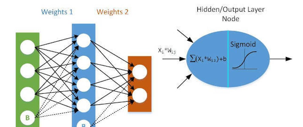
fan_in : Number of inputs to the neuron
fan_out : Number of outputs to the neuron

In the above image the fan_in=5, fan_out=3
Now the question can arise like we should only take fan_in and fan_out to define number of inputs and number of outputs ?
The answer is no, you can define any expression of your choice .For the explanation I have used the expression that are used by the researchers.
1)Uniform Distribution :
The Uniform distribution is a way to initialize the weights randomly from the uniform distribution.It tells that we can initialize the weights that follow Uniform Distribution criteria with the minimum value & maximum values.It works well for the sigmoid activation function.
The weight calculation will be :
Wij~D[-1/sqrt(fan_in),1/sqrt(fan_in)]
Where D is a Uniform Distribution
Code :
import keras
from keras.models import Sequential
from keras.layers import Dense
#Initializing the ANN
classifier=Sequential()
#Adding the NN Layer
classifier.add(Dense(units=6,activation='relu'))
classifier.add(Dense(units=1,kernel_initializer='RandomUniform',activation='sigmoid'))
# Summarize the loss
plt.plot(model_history.history['loss'])
plt.plot(model_history.history['val_loss'])
plt.title('model_loss')
plt.xlabel('epochs')
plt.ylabel('loss')
plt.legend(['train','test'],loc='upper left')
plt.show()
py
Here the kernel_initializer is RandomUniform
Epochs vs Loss function Graph :

2) Xavier/Glorot Initialization :
Xavier Initialization is a Gaussian initialization heuristic that keeps the variance of the input to a layer the same as that of the output of the layer. This ensures that the variance remains the same throughout the network.It works well for sigmoid function and it is better than the above method.In this type there are mainly two variations :
i)Xavier Normal :
Normal Distribution with Mean=0
Wij~N(0,std) where std=sqrt(2/(fan_in + fan_out))
Here N is a Normal Equation.
ii)Xavier Uniform :
Wij ~ D [-sqrt(6)/sqrt(fan_in+fan_out),sqrt(6)/sqrt(fan_in + fan_out)]
Where D is a Uniform Distribution
Code :
import keras
from keras.models import Sequential
from keras.layers import Dense
#Initializing the ANN
classifier=Sequential()
#Adding the NN Layer
classifier.add(Dense(units=6,activation='relu'))
classifier.add(Dense(units=1,kernel_initializer='glorot_uniform',activation='sigmoid'))
# Summarize the loss
plt.plot(model_history.history['loss'])
plt.plot(model_history.history['val_loss'])
plt.title('model_loss')
plt.xlabel('epochs')
plt.ylabel('loss')
plt.legend(['train','test'],loc='upper left')
plt.show()
py
Here the kernel_initializer is glorot_uniform/glorot_normal
Epochs vs Loss Function Graph :

3)He Init :
This weight initialization also has two variations. It works pretty well for ReLU and LeakyReLU activation function.
i)He Normal :
Normal Distribution with Mean=0
Wij ~ N(mean,std) , mean=0 , std=sqrt(2/fan_in)
Where N is a Normal Distribution
ii)He Uniform :
Wij ~ D[-sqrt(6/fan_in),sqrt(6/fan_in)]
Where D is a Uniform Distribution
Code :
#Building the model
import tensorflow as tf
import keras
from keras.models import Sequential
from keras.layers import Dense
from keras.layers import PReLU,LeakyReLU,ELU
from keras.layers import Dropout
#Initializing the ANN
classifier=Sequential()
#Adding the input Layer and the first hidden Layer
classifier.add(Dense(units=6,kernel_initializer='he_uniform',activation='relu',input_dim=11))
classifier.add(Dense(units=6,kernel_initializer='he_uniform',activation='relu'))
classifier.add(Dense(units=1,kernel_initializer='glorot_uniform',activation='sigmoid'))
classifier.compile(optimizer='adam',loss='binary_crossentropy',metrics=['accuracy'])
y_pred=classifier.predict(X_test)
y_pred=(y_pred>0.5)
py
Here the kernel_initializer is he_uniform/he_normal
As we come to an conclusion. While I was working on Churn Modelling problem I tried the above mentioned weight initialization techniques and able to find which technique is best for each activation function like relu,sigmoid.I have attached the dataset for your reference Churn Modelling dataset
The weight initialization techniques is not limited to the above mentioned three. But the above mentioned three methods have been widely used by the researchers.


Latest comments (0)