How I am learning machine learning - week 9: evaluating a model in scikit-learn (part 1)

in the last posts, we saw that the evaluation of a model was just getting the accuracy of predicting the target column for then calculating the average of them, but there is more. In this article, we'll begin to dive deep into one of the most important parts of a machine learning project: the evaluation of a model.

table of contents:

• The method of every model
• The scoring parameter
  • The cross-validation score
  • Comparing cross-validation estimator and score method
• The roc curve

The method of every model

If you are a bit skilled in programming you have probably noticed that a model is just an object which we called some methods on, mostly fit and score. If we look at the documentation we can notice that using the score method is the most basic way to evaluate our model: we divide our dataset into training and test, use training for training, test for testing, and, lastly, see how much accurate was the model into predicting the test.

The scoring parameter

Till now we have used the score method, which requires the splitting of our dataset into training and testing for then evaluating the mean results of their accuracy:

from sklearn.model_selection import train_test_split

...

x_train, x_test, y_train, y_test = train_test_split
model.fit(x_train, y_train)
model.score(x_test, y_test)

but the scoring method uses the cross-validation score. Let's try it in on the iris datasets that we already saw:

It returns 5 values and takes as arguments our model, the x and y-axis for then an unknown last argument: cv. How does it work?

The cross-validation score

using the score method it may happen to have a lucky score where the accuracy is higher than it should be, the n-fold cross-validation score works in a way to minimize it:
<!-- photo 3 -->

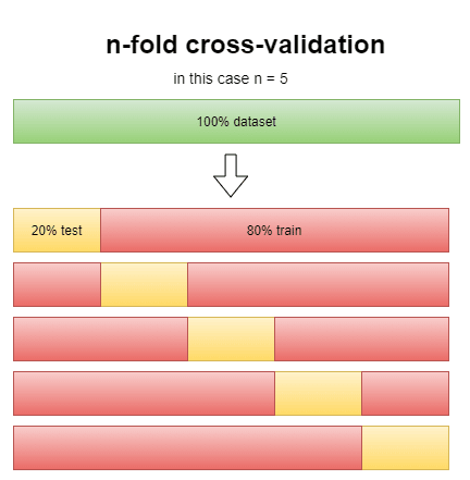
this way we reduce by a lot the possibility of a lucky score. The "cv" argument in the function stands for the n in n-folds, but to see how effective it really is can we compare the score method with the cross-validation estimator.

Comparing cross-validation estimator and score method

to compare cross-validation with the score method we can simply calculate the mean of all the values that it returned:

# calculating the accuracy with the score method
clf_score = clf.score(x_test, y_test)

# calculating the accuracy with the cross-validation estimator
cross_values = cross_val_score(clf, x, y, cv = 5)
clf_cross_val = np.mean(cross_values)
clf_score, clf_cross_val

and the scoring parameter?

But in the cross-evaluation method, you may have noticed something: where is the scoring parameter? It is an argument into the function that is initially set on None. When on None, it uses as scoring the mean accuracy of the model, the result of the score method.

The roc curve

in this series we have seen just the accuracy evaluation: how accurate is our model for predicting unknown data? Being the most basic metric is not the only one:

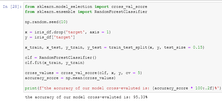
footnote: the accuracy is calculated as a parameter between 0 and 1, that's why in the presentation (the print function) we did accuracy_score * 100:.2f. the multiplication transform 0.9533 into 95 and :.2f at the end simply print the last two floating numbers "33". it's a way to format text in python.

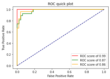
The ROC curve is a type of graph used to measure the usefulness of a test in general. It uses the true positive rates (tpr) and the false-positive rates (fpr) to show the trade-off of a particular subject. The most classical example can be done with a model that has to predict if the patients in a hospital have a disease (1) or not (0):

• if the model predicts 1 and is 1: true positive
• if the model predicts 1 and is 0: false positive
• if the model predicts 0 and is 1: false negative
• if the model predicts 0 and is 0: true negative

Usually, the ROC curve is used for binary classification. To use it on our iris dataset, which has 3 classes to classify, it's better to use the OneVsRest classifier, a type of model dedicated to fitting data in this cases. This classifier has methods in it that let us make a ROC curve for a non-binary classification. The code will be:

from sklearn.svm import SVC
from sklearn.datasets import load_iris
from sklearn.metrics import roc_curve, auc, roc_auc_score
from sklearn.model_selection import train_test_split
from sklearn.preprocessing import label_binarize
from sklearn.multiclass import OneVsRestClassifier

# initializing our axes 
x = iris_df.drop('target', axis = 1)
y = iris_df['target']

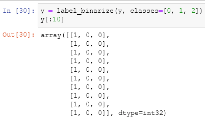
# Binarizing the output (the target column)
y = label_binarize(y, classes=[0, 1, 2])
# the numbers of classes are the second dimension of the array
n_classes = y.shape[1]

# splitting into train and set the data
x_train, x_test, y_train, y_test = train_test_split(x, y, test_size= 0.5)

# using as clf the OneVsRest, it fit one clf per class
# and fit the class against the others
clf = OneVsRestClassifier(SVC()) # as estimator is uses the Support Vector Classificator
# the tpr score of y is estimated by decision_function,
# which tells us how far we are amd which side we are on 
# the plane generated by the classifier
y_score = clf.fit(x_train, y_train).decision_function(x_test)

# making them a dictionary we ca, all the curves that we need
fpr = dict()
tpr = dict()
roc_auc = dict()
for i in range(n_classes):
    # the roc_curve function returns the fpr, the tpr and the thresholds
    # writing array[:, i] will return the tpr of that array
    fpr[i], tpr[i], threshold = roc_curve(y_test[:, i], y_score[:, i])
    # calculating the area under the ROC curve
    roc_auc[i] = auc(fpr[i], tpr[i])

in the begin, we imported all the libraries that we need and their usefulness. the initialization of our axis is something that we already did a lot of times. The binarization of the y-axis is used to extend regression and binary classification algorithms to multiclass classification ones, it takes an array (the y-axis or the target column) and another array that holds the classes of the y-axis: in this case, we have just three types of flower and the array will be [1, 2, 3]. n_classes is just the total number of the classes which is the same of the second dimension of the binarized array. A binarization of an array is similar to the one-hot encoding that we already saw:

splitting our data into training and testing is, again, something that we already know. The OneVsRest classifier, also known as one-vs-all, fit every class against the other, fitting one classifier per class. It takes as an estimator another model. In this case, we used the Support Vector Classification which handles the multiclass one-vs-one scheme going in synergy with the OneVsRest.
The calculation for y_score is already commented in the code but for more information, you can go here. Then we create the variables fpr, tpr and auc_roc as dictionaries so that we can store multiples values. For the iteration we have to take a step back: to calculate a single ROC we would write fpr, tpr, threshold = roc_curve(y_test[:, 1], y_score[:, i]) where the roc_curve function returns three values: the fpr, the tpr plus the threshold, and takes as argument two arrays in a very strange way: y_test[:,1] and y_score[:,1]. This is the syntax to extrapolate the true positive rate from the array that we have treated in this way, doing the same with normal python/numpy arrays would result in an error.
In this case we have three classes and that mean that we have to calculate the ROC three times and store them into three different memory area, that's why the loop:

fpr = dict()
tpr = dict()
roc_auc = dict()
for i in range(n_classes):
    fpr[i], tpr[i], threshold = roc_curve(y_test[:, i], y_score[:, i])
    roc_auc[i] = auc(fpr[i], tpr[i])

To know the score of Area Under the ROC Curve we can use the dedicated function roc_auc_score:

at the end of all of this we did a lot of calls and to see the results we have to plot the ROC curve. I've made a function to plot it quickly based on the documentation:

%matplotlib inline
import matplotlib.pyplot as plt

def plot_roc(fpr, tpr, n_classes):
    """
    takes two dictionary  one about the fpr and tpr plus the 
    number of classes for then doing a quick plot of all of them.
    can be a lot better, still a great starting point
    """
    # for now max three colors
    colors = ['red', 'green', 'orange']
    plt.figure()
    for i in range(n_classes):
        plt.plot(fpr[i], tpr[i], color=colors[i],
        label='ROC score of %0.2f' % roc_auc_score(y_test[:,i], y_score[:,i]))
    #creating the guessing baseline
    plt.plot([0, 1], [0, 1], color='navy', linestyle='--')
    plt.xlabel('False Positive Rate')
    plt.ylabel('True Positive Rate')
    plt.title('ROC quick plot')
    # positioning the legend
    plt.legend(loc="lower right")
    plt.show()

plot_roc(fpr, tpr, n_classes)

And now we can see the results:

Last thoughts

This week we saw an initial way on how to evaluate a model using scikit-learn, next week we'll see other ways like the confusion matrix. If you have any doubt or critic feel free to leave a comment.