How I am learning machine learning - week 8: basic models in scikit-learn

Last week we saw how to clean our data, so now we should be ready to see some machine learning model. The most basics are the regression to predict a number and classification to predict a category.

Table of contents:

• Importing a scikit learn toy dataset
• Using a regression model
• Classification models
• Overview of the random forest logic

Importing a scikit learn toy dataset

A machine learning algorithm is usually called a model or estimator and scikit-learn offers us a cheat-sheet with everything we can use:

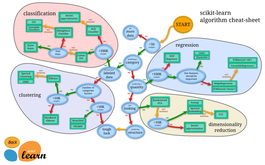
In our case, we already know that we want to try a regression estimator, but this cheat-sheet will come in hand very often.

Let's begin with importing one of the sample datasets that scikit offers:

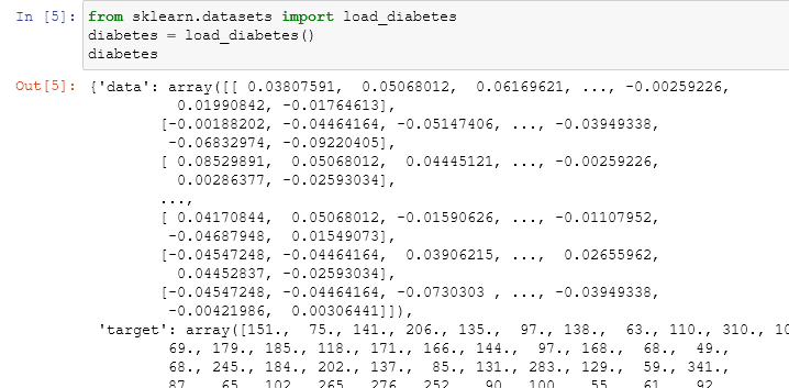
from a quick look we can understand that this is a dictionary with four important keys:

• data: a numpy array with a multidimensional shape that contains all our data
• target: a series that contains the values that we'll predict
• feature_names: the names of every column corresponding to the shape of the data.
• DESCR: a description of our dataset.

note that this is a toy dataset, usually, our data will not come with all this information in handy

to import it and use it our code will be similar to:

# importing the sample dataset
from sklearn.datasets import load_diabetes
# assigning it to a variable
diabetes = load_diabetes()
# reading the dataset description
print(diabetes.DESCR)

and the result will be:

Now, to convert the dictionary into a dataframe we have to first transform it into a pandas dataframe and we can do it easily with the functions that we already know:

diabetes_df = pd.DataFrame(diabetes['data'], 
                           columns = diabetes['feature_names'])
diabetes_df['target'] = pd.Series(diabetes['target'])
diabetes_df.head()

Using a regression model

now that we have everything prepared we have to simply import the regression model that we need. So, based on the cheat-sheet, let's try the ridge model:

# importing the model
from sklearn.linear_model import Ridge

# setting up the seed 
np.random.seed(10)

# creating the data
x = diabetes_df.drop('target', axis = 1)
y = diabetes_df['target']

# splitting the data
x_train, x_test, y_train, y_test = train_test_split(x, y, test_size = 0.15)

# instantiating the model
model = Ridge()
model.fit(x_train, y_train)

# checking up the score of the model
model.score(x_test, y_test)

in this case, the output will be:

0.5011092582547553

Now let's see in detail what we did: we first import the model and set up the seed with numpy, we split our data into train and test for then arriving at the clue part, the fit and the score functions.
We create the model variable and assign to it the Ridge() model, on the model we apply first the fit method. In machine learning fitting equals training. The training process finds the coefficients of the model equation, in this case, regression.
The score method evaluates the accuracy score of the model for then printing it on the screen.
In the notebook, all of this be:

In this case, we have very low accuracy but, strangely enough, using a better model, the random forest regressor, we'll still have low results:

Optimizing our models is something we'll see later on. It works, and this is already a great starting point.

classification models

Let's import another toy dataset from the one that scikit learn offers to see some classification models:

after viewing the dictionary we can see that there isn't an array with the name of our columns but only an array with the corresponding string of what every target should be.
We'll have to do a bit of manual labor:

column_names = ['sepal length', 'sepal width', 'petal length', 'petal width']
iris_df = pd.DataFrame(iris.data, columns = column_names)
iris_df['target'] = iris['target']
iris_df.head()

and the result will look like this:

but the numbers in the target column are confusing and it is not efficient to go back and forth to see what a category a number indicates, this was my solution:

# changing target values with strings
iris_df['target'] = iris_df['target'].astype(str)

for i in range(len(iris_df['target'])):
    if iris_df['target'][i] == '0':
        iris_df['target'][i] = iris.target_names[0]
    elif iris_df['target'][i] == '1':
        iris_df['target'][i] = iris.target_names[1]
    elif  iris_df['target'][i] == '2':
        iris_df['target'][i] = iris.target_names[2]

this is the moment when we should convert our dataframe with one-hot encoding, but with the latest versions of scikit, we can even do not do it. Previously it would have thrown an error, now works without problems.

Everything is ready, we have to just train our model on the data, so let's try the random forest classifier:

# importing the random forest classifier estimator
from sklearn.ensemble import RandomForestClassifier

# set up random seed
np.random.seed(10)

# make the data
x = iris_df.drop('target', axis = 1)
y = iris_df['target']

# split the data
x_train, x_test, y_train, y_test = train_test_split(x, y, test_size = 0.15)

# instantiate random forest
clf = RandomForestClassifier() # clf is short for classifier
clf.fit(x_train, y_train)

# evaluate random forest
clf.score(x_test, y_test)

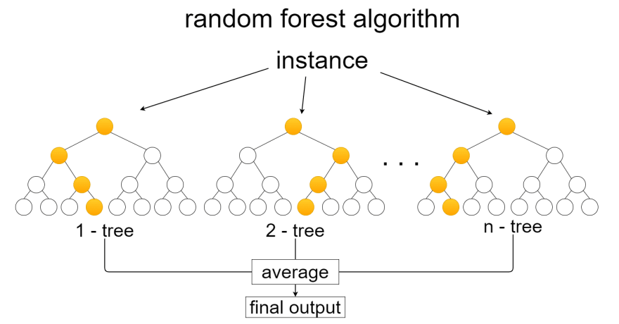
overview of the random forest logic

Now we have successfully used our model to predict the flower categories. We used the random forest classifier and regressor, two algorithms that have a simple logic behind them that makes them highly effective: they build and train various decision trees to then output the average of their decisions.

We can use the predict and predict_proba functions to see what we are doing a bit further.
the predict function output the vote of the trees. If used for the first 5 samples of x_test it will return the decision of what every target should be:

but every prediction isn't 100% accurate and every sample has a probability of being a class or another one. the predict_proba function shows us this probability in detail:

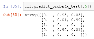
It returns an array with all the data in it. For classification, every element of the array is a nested array with the probabilities in it. our possible cases are in order: Setosa, Versicolour, and Virginica. If we look at the top of the output we can see three numbers where everyone corresponds to the probability of a plant being a specific type: in the first case there is a probability of 0% that the plant is Setosa, 95% of it being Versicolor and 5% of it being Virginica, the prediction will then be Versicolor, and if we see the precedent figure we can see that the target of the test is Versicolor.

Last thoughts

This week we saw the basics of classifications and regression models for then having an overview of how they reach a result, next week we'll talk about evaluation.