
Introduction
The first blog post of the RUM series introduced the RUM conjecture. It describes the trade-off between read (RO), update (UO), and memory (MO) overheads that one should take into account when designing data structures and access methods.
In this post we want to take a closer look at data structures designed for low update overhead that are commonly used in practice, i.e. logs and journals, log-structured merge-trees, as well as B trees and some B tree extensions.
This blog post is the third part of the RUM series:
- RUM Conjecture - Reasoning About Data Access
- Read Efficient Data Structures
- Update Efficient Data Structures
- Memory Efficient Data Structures
In order to compare the different implementations we are using the same example as in the other posts. The task is to implement a set of integers, this time focusing on a small update overhead.
The post is structured as follows. In the first section we want to recap the solution from the opening post which has minimum update overhead. The next section reveals how the update-optimal solution, also known as logging or journaling, can be adopted in real-life scenarios. The third section introduces the concept of log-structured merge-trees (LSM trees), a class of data structures combining the idea of an immutable log and read efficient data structures. The following section briefly discusses B trees as they play a major role in database indexes but also for LSM trees. The last but one section is going to shed light on practical implications when choosing a database implemented on top of LSM trees. We are closing the post by summarizing the main points.
Update-Optimal Solution
The simplest way to achieve constant (and minimal) update overhead, is to append each update to a transaction log. Taking the use case where we want to implement a set of integers, we store insertion and deletion operations in a sequence, always appending the latest one. As point queries potentially have to go through the complete log, which might also grow indefinitely, we derived the following RUM overheads:
- RO → ∞
- UO = 1
- MO → ∞
In contrast to the read-optimal solution, the update-optimal method is actually used in practice. Depending on the context, it is refered to as logging or journaling.
Log / Journal
Concept
The following picture illustrates how the set {0..6} could look after a few update operations.
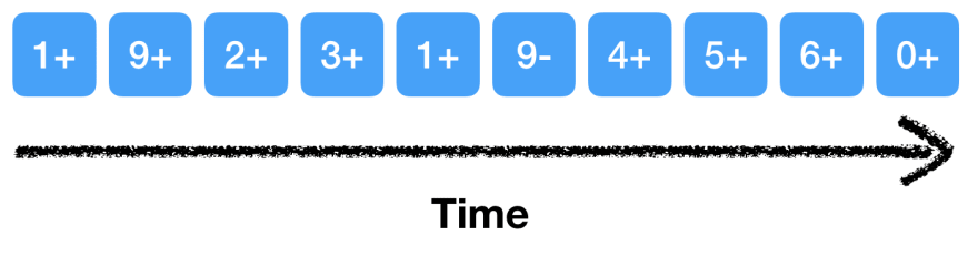
Writes are sequential as we only append new data, keeping the rest of the log untouched. It has been shown that sequential writes on disk are comparable or even faster than random access in memory. [1]
What is the use case for logging / journaling? The longer a log exists, the poorer its read and memory overheads become.
The bad read performance of this very simple data structure can be compensated in two ways (or a combination of both). First we can limit the amount of reads on the log by reading the log only once sequentially, transferring the data to more read-efficient data structures, e.g. trees, asynchronously.
Databases like PostgreSQL are storing transactions in a write-ahead-log file. Using direct IO to bypass the page cache in combination with appending to the log minimizes the time until the database can acknowledge the transaction without the risk of losing data. Then it can asynchronously go through the log, applying transactions to the actual tables. The log is only read once when it gets applied. In case of a crash, the database can also use the log to replay the transactions that have not been executed, yet. Utilizing the write-ahead-log gives us durability and atomicity without sacrificing throughput.
Another very similar use case is in journaling file systems (JFS). In JFSs, changes are first stored in the journal before they are applied to the main filesystem structure.
Secondly we can avoid searching the whole log by building up an index which contains the log file offset for certain transactions or messages. While this is not practical for our integer set example, as the index would not be much smaller than the actual data, it is used in message queue systems, e.g. Apache Kafka, which rely on high message throughput and consume messages only sequentially.
How can we deal with the potentially indefinitely growing memory overhead? One option is to impose limits on the log. Kafka allows the user to configure either time (log.retention.hours) or size (log.retention.bytes) based retention policies.
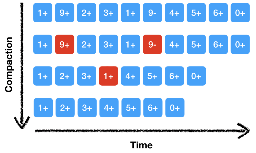
Another commonly used technique is called compaction. Looking at our set example from above, storing the information that a value has been deleted from the set is only necessary if it has been added before. During compaction we remove transactions that do not affect the final state.
The following diagram illustrates how we can reduce the size of our integer set from above using compaction. We are removing redundant transactions, leaving a shorter log. Compaction can be performed based on a time or space constraint.
RUM Overheads
In the simplest implementation of a log without any compaction, retention, or indexing, the RUM overheads are the same as in the update-optimal solution. In a log of size m, we have at most m read operations until we find whether a value is a member of the set. Update overhead is 1, as we only append. Memory overhead will grow indefinitely unless a retention policy is in place. Compaction can help to reduce the memory overhead as well.
Asymptotic Complexity
The asymptotic complexity directly corresponds to the RUM overheads. We get linearly growing read and memory requirements depending on the log size, while having constant update complexity in both the average and worst case. If we perform regular compaction, we can keep the number of transactions m close to the number of integers n.
| Type | Average | Worst case |
|---|---|---|
| Read | O(m) | O(m) |
| Update | O(1) | O(1) |
| Memory | O(m) | O(m) |
Researchers and database developers have spent a huge amount of time combining logs with other data structures and techniques to compensate the bad read and memory overhead. A frequently used type of update-efficient data structures that combine logging and indexing are so called log-structured merge-trees.
Log-Structured Merge-Tree
Concept
Log-structured merge-trees (LSM trees) [2] are more a framework on how to combine different levels of data structures rather than an actual data structure. They address the problems of append-only logs discussed in the previous section on a conceptual level which we are going to look at in this section. The actual performance of LSM trees heavily depend on the concrete implementation and data structures used.
The main idea of LSM trees is to maintain a hierarchy of data structures, each of which is optimized for the underlying storage medium. In a two-level LSM tree the first level is typically stored in memory, while the second level is stored on disk. The following figure illustrates the concept of a two-level LSM tree.

The original paper proposes to use B tree like structures for the individual trees. This is useful as we can adjust the node size to the block size of the file system. However as the first level resides in memory, we can use other self-balancing trees as 2-3 trees or AVL-trees alternatively.
Databases like Bigtable [3] or Apache Cassandra [4] do not actually store higher levels as trees but in the sorted-string table (SSTable) file format. An SSTable is a file of key-value pairs, sorted by key. It is also common to store a mapping from key to offset in the data file in addition.
As discussed earlier, when storing the first level in-memory, we typically persist updates to a simple write-ahead log to ensure durability. Read queries first hit the in-memory level, which is a read efficient data structure. If the key is not found, we proceed with the next level. In order to avoid scanning all the levels we can use approximate indexes, e.g. bloom filters, to determine whether a key is included in parts of the LSM trees.
Updates are performed in-place in the in-memory level. This is not a problem as RAM is sufficiently fast for random access and we can acknowledge the transaction as soon as we hit the write-ahead log. When the in-memory level is full we persist to the next level. If we are using B trees across all levels, it can simply persist the tree as it is. In case of SSTables we store the records as sorted key-value pairs and add an index if required.
The disk-based updates will eventually fill up the disk. This is where compaction comes in handy again. From time to time we can merge the different trees / SSTables, effectively reducing the total size. After a successful merge we can discard the outdated data. This is also where the name log-structured merge-tree is derived from. We are storing updates in a log of trees, merging them in order to compact, reducing the impact of growing read and memory overhead.
RUM Overheads
The actual RUM overheads of LSM trees are heavily depending on the concrete implementation. They correspond to the RUM overheads of the different levels. We also have to take the effort of persisting one level to the next one and the overhead of merging in case of compaction.
Asymptotic Complexity
Naturally the asymptotic complexity also depends on the actual implementation and data structures used. If we keep the data as compacted as possible, we can achieve logarithmic read performance in terms of actual elements in the set n rather than transactions m, given we use sorted data structures for all levels. The update complexity will correspond to the in-memory data structure. However if we use a write-ahead log we can make it seem like constant time.
If the database load gets high and it receives many queries at the same time the performance goes back what a normal log can guarantee. Some implementations, e.g. SwayDB, provide back-pressure mechanisms if compaction cannot keep up.
We now understand why LSM trees are a powerful tool for databases aiming at superior update performance. As the original LSM tree paper suggests to use B tree like structures for individual levels, we want to take a quick look at B trees in the next section.
B Trees
Concept
B trees [5] are a generalization of self-balancing binary search trees where a node can have more than two children. For every node the left sub-tree contains only elements that are smaller than the current value, giving us logarithmic search complexity. The following picture illustrates a B tree with maximum block size of 4 holding the set {0..6}.

B trees have the same asymptotic read, update, and memory complexity as binary search trees. So why do we mention them in an article about write efficient data structures?
In B trees you can tune the number of elements stored in a node to fit the block size of your filesystem or sector size of your hard disk, respectively. This makes them more suitable for storage on sequential storage mediums than regular binary search trees, e.g. the red-black trees from the previous post. Additionally, there are many extensions and derivations which focus on reducing the update overhead. B trees and extensions are widely used in databases and filesystem implementations.
Two B Tree Extensions
B+ Trees
Unlike B trees, B+ trees store records only in leaf nodes. While this extension is not very useful in our integer set example, it does heavily influence performance of databases where B+ trees are commonly used as indexes.
They are not particularly tuned for better update performance but allow higher branching factors than B trees as only keys are stored in intermediate nodes. This might enable us to store the all non-leaf nodes in memory, limiting disk I/O only to the times when database records have to be modified.
Additionally, B+ trees store pointers from one leaf node to the next one, speeding up queries spanning multiple leaf nodes significantly.
Fractal Trees
Fractal trees [6] have the same asymptotic read complexity as B trees. However they provide better update performance. This is achieved by maintaining buffers in each node, storing insertions in intermediate locations. This improves the worst-case performance of B trees where a each disk write might change only a small amount of data (see also write amplification).
Fractal trees are available as a storage engine for MySQL and MariaDB (see TokuDB), and MongoDB (see TokuMX).
RUM Overheads
The RUM overheads of a B tree depends on the branching factor and the current state of the tree. A search query has to start from the root node, performing binary search within the node to find the respective child pointer to follow. While we might have to follow less pointers than in binary search trees, we have to perform more comparison operations within a node. Thus the read overhead is proportional to the number of elements in the tree.
The update overhead is equal to the read overhead plus one operation to insert or delete an element. In order to keep the tree balanced we might have to split (insert) or merge (delete) a node. Similar to red-black trees this might affect larger parts of the tree.
The memory overhead is also proportional to the number of values stored within the tree. However we can reduce the memory overhead by increasing the maximum size of each node. This way we will have a smaller tree and have to store less pointers. We can also align the node size to the page size / block size of the machine.
Asymptotic Complexity
As mentioned above the asymptotic complexity is equivalent to the one of binary search trees.
| Type | Average | Worst case |
|---|---|---|
| Read | O(log n) | O(log n) |
| Update | O(log n) | O(log n) |
| Memory | O(n) | O(n) |
LSM Trees In Practice
Now that we have an overview of update efficient data structures, let's take a look at some numbers. For now I want to focus on LSM trees, as they are widely used in different databases. The following non-exhaustive list contains databases that use or support LSM trees for persisting data.
When choosing a database to handle persistence for you, it is not easy to pick the right product. After you decided for one you can either stick with the default configuration or try tuning it based on your needs.
I want to use a benchmark conducted by the developers behind SwayDB to visualize a few trade-offs when it comes to different configuration parameters. SwayDB is a highly configurable, type-safe and non-blocking key-value storage library for single/multiple disks and in-memory storage written in Scala. The numbers are taken from the tests run on a mid 2014 MacBook.
We are going to look at the read and write throughput (operations per second) in different scenarios.
- The first variable is whether the read and write operations are performed with keys in increasing order (sequential) or shuffled (random).
- The second variable is how the database is set-up. We are comparing a 2-level in-memory LSM tree, an 8-level memory-mapped file based LSM tree (
java.nio.MappedByteBuffer), and an 8-level regular file based LSM tree (java.nio.channels.FileChannel).
In-memory data structures are fast, but not durable. Memory-mapped files give durability and read and write performance but since they do not guarantee writes on fatal server crashes, they are not as durable as regular file access. Maximum durability can be achieved using direct IO, but I am not sure if this can be configured in SwayDB.
First let's take a look at the influence of the compaction process on the database performance. The following chart compares the read throughput during and after compaction for random reads.

The compaction process slows down the database to around 50% random read performance, independently of the persistence configuration! Compaction is essential when using LSM trees to keep reasonably good read performance and avoid consuming too much space. However the compaction strategy should be chosen wisely as it might come at high price if it happens too frequently or not often enough.
A second question that is interesting is the impact of the key ordering on write performance. The next chart compares write throughput when using ordered keys and shuffled keys in the 2-level in-memory LSM tree.
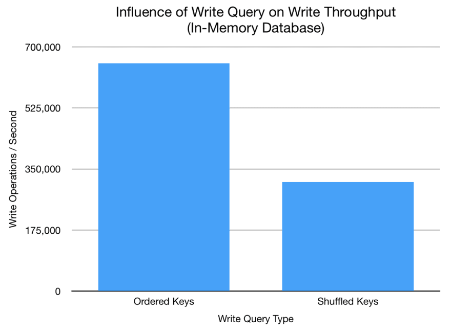
Amazing! We get around 100% speed-up when writes are ordered and not shuffled. This shows that depending on the query and data structure used, you can have quite significant performance differences. SwayDB uses skip lists under the hood and sequential insertion just appends to the end of the skip list, promoting the elements as needed. Random insertions however result in modifying and re-linking multiple elements and levels in the middle of the skip list.
Last but not least we want to investigate on the performance impact of trading durability for throughput. In the following chart we compare write throughput of shuffled and random writes for our 2-level in-memory, 8-level memory-mapped file based and 8-level regular file based LSM trees.

As expected, in-memory LSM trees offer the best performance. While regular file access gives the best durability it also has the worst performance. Memory-mapped files offer decent performance if data loss and a following recovery from the write-ahead log in case of a fatal crash is acceptable.
Summary
In this post we looked at the update-optimal solution, also known as logging / journaling, and how it is used in practice. We have seen that by maintaining a log of tree-like structures (LSM trees), we can achieve decent write throughput without sacrificing too much of read performance.
We also briefly introduced B trees as they play an important role in LSM trees and as database indexes. While B trees are not specifically designed to be update efficient there are extensions aiming at reducing write amplification, for example.
Last but not least we saw that tuning your database according to your needs can have significant performance impacts. When using LSM trees, topics like compaction and compression also play an important role.
Did you ever use a database which uses LSM trees to persist its state? What is the data structure used by your favourite database? Do you know any other extensions of B trees that aim at improving update overhead? How do they work? Let me know in the comments below! The next post is going to focus on space efficient data structures.
References
- [1] Jacobs, A., 2009. The pathologies of big data. Communications of the ACM, 52(8), pp.36-44. ACM Queue Post
- [2] O’Neil, P., Cheng, E., Gawlick, D. and O’Neil, E., 1996. The log-structured merge-tree (LSM-tree). Acta Informatica, 33(4), pp.351-385.
- [3] Chang, F., Dean, J., Ghemawat, S., Hsieh, W.C., Wallach, D.A., Burrows, M., Chandra, T., Fikes, A. and Gruber, R.E., 2008. Bigtable: A distributed storage system for structured data. ACM Transactions on Computer Systems (TOCS), 26(2), p.4.
- [4] Cassandra Documentation "How is data written?"
- [5] Comer, D., 1979. Ubiquitous B-tree. ACM Computing Surveys (CSUR), 11(2), pp.121-137.
- [6] Bender, M.A., Farach-Colton, M., Fineman, J.T., Fogel, Y.R., Kuszmaul, B.C. and Nelson, J., 2007, June. Cache-oblivious streaming B-trees. In Proceedings of the nineteenth annual ACM symposium on Parallel algorithms and architectures (pp. 81-92). ACM.
- Cover image from the Library of Congress, Prints and Photographs division. Digital ID fsa.8c35555. Public domain, https://commons.wikimedia.org/w/index.php?curid=543535


Top comments (7)
Thanks for this well written and comprehensive post. How do these data structures fare in terms of cache locality? I have heard that many libraries prefer radix trees as compared to B-trees because of the cost of L1-cache misses.
Thanks for the question! I am not that familiar with tries or radix trees. I know that are used as prefix trees for tasks like auto-completion.
But from what I can tell plain radix trees don't seem to be very cache-friendly. In a B-tree you have an array of values in each node, enabling prefetching for faster comparisons. But it seems that there are HAT-tries, an extension of radix trees, which have the same idea of storing an array of values in each node.
Do you have any link / reference to look at regarding the preference of radix trees over B-trees due to the cache behaviour? I'm curios and would love to read more :)
Regarding the cache-friendliness of the data structures presented here it depends on what you are doing. To me it seems that there is no single definition of "cache-friendly". An array is more cache-friendly than a linked list if you iterate. However when concurrently updating the data structure then a linked list allows for local modifications, reducing the amount of synchronization needed also in the cache.
Having said that, if you implement the log / journal in-memory as a linked list it will behave like a linked list. However in practice it is mostly persisted on disk, written once, such that cache friendliness is not that relevant. For LSM trees it depends on which data structures you use on each level.
Maybe someone else can also comment. Also please correct me if I'm wrong :)
I read it while looking up Judy Arrays. Their documentation is a little dated (circa 2000) but quite detailed. They mention specifically that 256-ary tree is very good in terms of cache-locality. Judy arrays are recommended to be used as sparse hash-tables though, so the use case is different from the one in your article.
What you said about cache-friendliness is true. I was thinking in terms of iteration.
Thank you for the link. I also found the post Hashtables vs Judy Arrays, Round 1 and it shows different scenarios in which either data structure excels.
It is safe to say that optimizing algorithms and data structures for the memory hierarchy, esp. CPU caches, is something where you can get a lot of performance boost. When I read Cache-Oblivious Algorithms and Data Structures I realized that there is a whole area of research around that and I know almost nothing :D
I think Data Engineering and my future are related, so I'll keep your series of articles in bookmark.
I found all the concepts separately, but not in relationship to the "real world", as in current products that use them, and not all technologies have white papers.
Glad to hear that you like Data Engineering and also that my posts are useful to you :)
I agree with you that it's sometimes difficult to figure out what data structures are used under the hood of different software products. If it is open source you can at least dig into the code. But the official websites mostly contain buzzwords and marketing figures.
If you want to know more about a specific product it's also useful to see if there are mailing lists, chats, or forums you can join. When working on this article I also talked to the developer of SwayDB, clarifying a few questions I had about the internals.
And one more thing. In case you don't know it already, there is an amazing collection of articles about the correctness and robustness of different databases and distributed systems: aphyr.com/tags/Jepsen I like to read this to get a different view on the technologies.
These posts take me like a week to get through (just dense and I have little time) but they are sooo worth it :D, thanks Frank!