Motivation
When reasoning about algorithm performance we often look at complexity. Especially when comparing different algorithms, looking at asymptotic complexity (e.g. the big-O notation) is useful. We have to keep in mind however, that the big-O notation "swallows" everything but the largest complexity factor. A prominent example where the big-O notation can be misleading is when finding a value in a collection. Hash maps are the default candidate for this use case, as the access to one particular element requires constant time. If you have only a few elements however, using a tree or even a simple list might be faster.
While you should look out for cases like this, there is another huge factor that influences performance: The computer hardware / architecture. Your CPU might be fast but it has to wait for I/O to finish. Your distributed algorithm might be powerful but your network topology does not suffice. In this blog post we are going to look at one particular part of the computer architecture which might impact algorithm performance in orders of magnitude: The memory hierarchy - and the CPU cache in particular.
The post is structured as follows. First we are going to look at a very popular example where the runtime performance is heavily influenced by the CPU cache utilization. The second section will give some theoretical background about computer architecture, allowing the reader to understand what is happening in the example. Afterwards we are going to revisit the example from the first section with the newly acquired knowledge. We are closing the blog post by summarizing the main ideas.
The Matrix Multiplication Example
The Formula
The example we want to use is a very basic one: Matrix multiplication. Matrix multiplication is used in a lot of places, e.g. image processing, AI, robotics, data compression. For multiplying the matrices A * B = C, the formula is as follows:
For each element of the result matrix, it goes row-wise through A and column-wise through B, multiplying each pair of elements, adding up the results. There is also a nice visual representation of the formula:
Now let's look at two different variations of this algorithm and measure the execution time for different matrix sizes. For simplicity reasons we are using two square matrices. They are filled with randomly generated double values.
We are using ScalaMeter for measuring the runtime performance. Feel free to check out my last blog post which contains more details about the tool.
The Experiments
Algorithm 1
The first algorithm is a naive implementation of the formula above. For two square matrices of size n it has to perform n³ multiplications and additions, thus having O(n³) complexity.
def mult1(m1: Array[Array[Double]],
          m2: Array[Array[Double]],
          size: Int): Array[Array[Double]] = {
  var res = Array.fill(size)(new Array[Double](size))
  var i = 0
  while (i < size) {
    var j = 0
    while (j < size) {
      var k = 0
      while (k < size) {
        res(i)(j) += m1(i)(k) * m2(k)(j)
        k += 1
      }
      j += 1
    }
    i += 1
  }
  res
}
Algorithm 2
The second algorithm transposes the second matrix before applying a slight variation of the formula, which has the indices of the second matrix within the multiplication inverted. For two square matrices of size n it first has to perform n² copy operations and then again n³ multiplications and additions. This also leads to O(n³) complexity, but with more overhead.
def mult2(m1: Array[Array[Double]],
          m2: Array[Array[Double]],
          size: Int): Array[Array[Double]] = {
  var m2t = Array.fill(size)(new Array[Double](size))
  var x = 0
  while (x < size) {
    var y = 0
    while (y < size) {
      m2t(x)(y) = m2(y)(x)
      y += 1
    }
    x += 1
  }

  var res = Array.fill(size)(new Array[Double](size))
  var i = 0
  while (i < size) {
    var j = 0
    while (j < size) {
      var k = 0
      while (k < size) {
        res(i)(j) += m1(i)(k) * m2t(j)(k)
        k += 1
      }
      j += 1
    }
    i += 1
  }
  res
}
The Results
Looking at both algorithms an educated guess might be that the first one is faster than the second one, as they are almost identical except for the transpose operation and the inverted indices. The relative difference between the two should decrease as the size increases, as n³ grows faster than n², which is also reflected in both algorithms having the same asymptotic complexity. The memory requirements of mult2 are a bit higher however, as it needs to transpose the matrix first.
Let's look at the execution time of both implementations for different matrix sizes n. We are also adding a column indicating the speedup (mult1 / mult2 - 1) you get when choosing the second implementation.
| n | Time mult1 (ms) |
Time mult2 (ms) |
Speedup |
|---|---|---|---|
| 10 | 0.011 | 0.014 | -20.5 % |
| 50 | 0.166 | 0.128 | 29.6 % |
| 100 | 1.307 | 1.102 | 18.5 % |
| 500 | 242.1 | 147.4 | 64.2 % |
| 1000 | 9 347 | 1 244 | 651.2 % |
| 3000 | 398 619 | 33 846 | 1077.7 % |
Impressive! Even though we are doing extra work, we are more than 10 times faster using mult2 for n = 3000! What is happening?
Before I am going to explain, it is useful to have some basic knowledge in computer architecture. The next section is going to cover that part. In case you are already familiar with that or cannot wait for the answer, feel free to skip the next section and revisit it later.
Computer Architecture
Von Neumann Architecture
Most of the modern computers, especially in the commodity segment, are based on the Von Neumann Architecture. Originally described in 1945 it evolved over time to what we have today. It describes the basic components of a computer, such as CPU, memory, and I/O devices, as well as how they are working together.
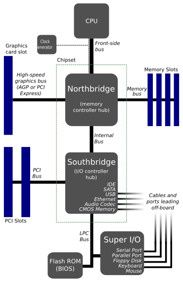
The following scheme depicts the main components and how they are connected. The central processing unit (CPU) is responsible for doing the computational work, e.g. arithmetic operations. It is connected to the main random access memory (RAM) through the northbridge. The northbridge also connects other high speed interfaces but we are not going to go into details here. If data is not available within memory, it has to be loaded from persistent storage. The different interfaces for this (e.g. IDE, SATA, USB) are connected through the southbridge.
This means that there is no direct connection from the processor to the data. If the data is in the main memory, it has to go through the northbridge, if it is not there, it also has to go through the southbridge. This storage hierarchy is necessary as there is a trade-off between storage cost, speed and size.
Storage Hierarchy
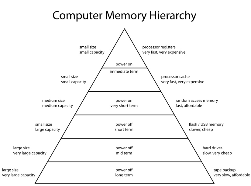
Storage can be categorized into persistent and volatile storage. In order for data to survive a reboot of the computer, it needs to be stored persistently, e.g. in a hard disk drive (HDD) or a solid state drive (SSD). The disadvantage of this storage is that is often not optimized for random access (which is fine for files but might not be for individual data or code). It is also very far from the CPU, which adds additional transfer latency.
When booting the operating system all required data is loaded into the volatile main memory. If the computer has no power the data will be lost. Also the main memory is typically much smaller. However, it is faster, especially in terms of latency, and it is optimized for random access.
While using the RAM for more frequently used data is a good idea, it is still not optimal as the CPU needs to go through the northbridge to read or modify the data. To overcome this problem, another layer of memory has been added to computers: The CPU cache.
Commodity main memory is typically based on dynamic RAM (DRAM). Consisting of fundamentally only one transistor and one capacitor per element, DRAM is cheap and can be packed very well, allowing for more capacity. However, due to its design it is much slower than static RAM (SRAM), which is typically used when even lower latency is required. SRAM is used in CPU caches. The following diagram summarizes the storage hierarchy we were discussing.
The CPU caches themselves typically also have different layers, reaching from the fastest but smallest level 1 (L1), up to the biggest but slowest level 3 (L3) cache. Additionally the L1 cache is devided into one part for data (L1d) and one for instructions / code (L1i).
If you have a multi-core CPU, some of the caches are shared between cores. If hyperthreading is enabled, the actual cache size heavily depends on the program you are executing as both hyperthreads have to share the same cache. For more details on this topic I recommend to take a look at the awesome paper What Every Programmer Should Know About Memory by Ulrich Drepper.
To give the reader an impression on the actual size of the different layers, the following table contains the specifications of my 2016 laptop.
| Storage | Size |
|---|---|
| L1i Cache | 32 KB |
| L1d Cache | 32 KB |
| L2 Cache | 256 KB |
| L3 Cache | 4 MB |
| Main Memory | 16 GB |
| SSD | 500 GB |
CPU Cache Usage
The cache stores data copies of frequently used main memory locations. While storing something on disk or in memory is a deliberate decision of the programmer, what is stored in the cache is mostly managed behind the scenes.
Data is transferred between main memory and cache in blocks of fixed size, so called cache lines. A cache entry contains the data as well as the memory location it caches. Whenever the CPU needs to access a memory location, it first checks the cache for a corresponding entry. If the entry exists, it is called a cache hit, otherwise a cache miss.
Cache hits are generally what you want because it avoids the (relatively) expensive main memory access. Note that you cannot avoid cache misses and they are not generally a bad thing. If a memory location is accessed for the first time, a cache miss is natural.
Modern CPUs, however, have mechanisms to avoid cache misses also in this situation. The processor has a small module responsible for prefetching cache lines. One example is when working with structural types, e.g. a person, and accessing one attribute of the person, e.g. the address, it is likely that you are going to access another attribute later. So the CPU will prefetch also other attributes, e.g. the age and name. Another example is sequential access on arrays. When accessing the first element of an array, the CPU will prefetch more elements in parallel while still dealing with the first one.
With this knowledge in mind, we want to go back to the original example of matrix multiplication and analyze why mult2 performed so much better for bigger matrices than mult1.
Matrix Multiplication Revisited
In the initial example we had two implementations for matrix multiplication: mult1 and mult2. Both were fundamentally the same, except that mult2 transposed the second matrix before entering the three nested loops performing the computation. But why does it make a difference? And why is is this difference only visible for bigger matrices?
Before we analyze the difference from a more theorical perspective, let's look at more numbers. We are going to execute both implementations again with different matrix sizes. This time we are not measuring the runtime, however, but instead we are looking at the CPU counters for L1d cache misses using perf.
for s in 10 50 100 250 500 1000 1500 2000 2500 3000
do
  for m in 1 2
  do
    # Run mult$m with size $s and record CPU counters
    perf stat -e L1-dcache-loads,L1-dcache-load-misses \
      java -jar cpumemory.jar $s $m
  done
done
What you can see is that starting with n >= 250, the L1d cache miss percentage increases for mult1. This means that the CPU has to fall back to the bigger but slower L2 cache. It wastes cycles, waiting for the required data to be available from higher level memory. But why is this the case?
As explained in the previous section, the CPU is prefetching data to the cache. That means when accessing the first element of the matrix, it is going to prefetch more elements in parallel. Recap the three nested loops with the three indices i, j, and k.
The first access of m1(i)(k) will trigger prefetching more elements, e.g. m1(i)(k + 1). The first access of m2(k)(j) as in mult1 however, is going to trigger prefetching m2(k)(j + 1). While this is not a big problem as long as the whole matrix fits into the cache, it becomes one with bigger matrices.
The inner-most loop increments k, and not j. So by the time j gets incremented, m2(k)(j + 1) might have already been evicted. This is the reason why mult2 performs so much better with bigger matrices. By transposing the matrix and then swapping the access to m2t(j)(k), even if the cache is full and parts of the matrix have to be evicted, we at least prefetch correctly for the inner loop.
Final Thoughts
In this blog post I was trying to show you why it is important to know some basics about computer architecture as a software developer. While most university grade computer scientists should learn this during their studies, it is certainly a good idea for everyone else who is writing code to read a bit more about this topic.
We looked at an implementation of the naive matrix multiplication algorithm where changing only a small detail lead to execution speed-up of over 1000%. It is important to note that mult2 is by far not the most optimal implementation. You can check out the paper Cache oblivious matrix multiplication using an element ordering based on the Peano curve for a cache optimized implementation that does not depend on the actual cache size. Also note that other algorithms having better asymptotic complexity than O(n³) exist, e.g. the Strassen algorithm.
Have you ever encountered a slow program that turned out to have a lot of cache misses? Did you use perf before? Do you think developers should be more aware of the cache logic in order to write efficient programs? Let me know your thoughts in the comments!


Top comments (7)
I totally agree with you! I feel that going down to the nitty gritty, learning about computer architecture, data structures, algorithms, and so on instead of just using a framework / library is super useful.
During my time at the university I had to choose between different courses and I always found it hard to do that. There is so much to learn. Luckily the internet is full of information and in CS most of the papers can be accessed free of charge.
Glad you liked it! Be sure to check out my other posts as well :)
Great post. I completely agree with Karim Manaouil on this one. However, when explaining why mult2 was faster than mult1, it might have been worth it to talk about spatial locality and how arrays are stored in memory. Still, thank you for writing about this.
Hey Ricardo,
Glad you enjoyed the post :)
You are right there are many details I did not talk about but they are equally important. Would you mind to elaborate a bit on the spatial locality and how arrays are stored in memory? I think that'd be super valuable for the discussion!
Thank you for commenting!
Sure :)
Simply put, spatial locality states that the data elements near an element that was just accessed have a high probability of being accessed as well. As for arrays, single dimension ones are stored in memory in a contiguous fashion (for arrays with more dimensions, you need to know the size at compile time, i.e. they have to be fixed size. If you don't know, the rows' elements are still stored contiguously, but there's no guarantee that the rows themselves will be close to each other. There are some tricks you can do with pointers to bypass this, though).
So, the caching process takes both of these ideas into consideration, being that contiguous array elements are usually cached together. This is why mult2 had a better performance - You were traversing the columns as if they were rows (which, as said above, are single dimension arrays). In other words, you were accessing contiguous elements in memory, and not jumping who knows how many memory addresses to access each element like in mult1. Hence the cache hits and cache misses on both examples.
Knowing this, some people even choose to represent their matrices through single dimension arrays. For instance, with a 2D matrix[10][10], you would have a single dimension matrix[100]. You would access each element through matrix[width * row + col], and thus, due to spatial locality and contiguous storage, take full advantage of your cache.
Hope that was clear :)
Yes but can you add memcached to make it faster?
At which point would you like to make use of memcached?
No, sorry, your profile picture is enough of an answer.