Excel Formulas to Sum columns based on Adjacent criteria!!

This page will guide you to learn the Excel formulas to sum or subtotal the values in adjacent columns based on certain criteria. Further, we will explain the formula syntax with a practical example. Let’s see them below!! Get an official version of ** MS Excel** from the following link: https://www.microsoft.com/en-in/microsoft-365/excel

General Formula:

• To sum the values in adjacent columns, use the below formula.

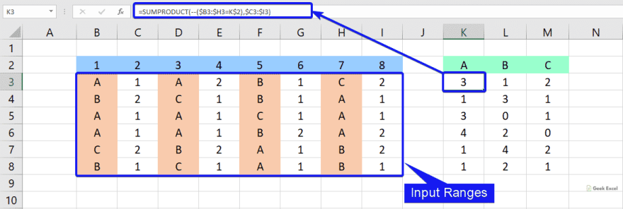
=SUMPRODUCT(–(range1=criteria),range2)

Syntax Explanations:

• SUMPRODUCT – In Excel, this function will help to multiply the corresponding array or range and returns the sum of the product. Read more on the SUMPRODUCT Function.
• Minus Operator (-) – This symbol will help to subtract any two values.
• Comma symbol (,) – It is a separator which helps to separate a list of values.
• Parenthesis () – The main purpose of this symbol is to group the elements.
• Range – It represents the input values given in the worksheet.
• Criteria -It is the condition that helps to sum the values.

Example:

• Now, we are going to see how to sum the values from adjacent columns.
• Refer to the below example.
• In the given image, we will enter the input values in Column B to Column I.
• Then, apply the given formula in the formula bar section.
• Finally, it will display the result in Cell K3 as per the below image.

Verdict:

From this tutorial, we guided you to learn the simple formulas used to sum the values in the adjacent columns based on certain criteria in Excel Office 365. Hope you like this article. If you have any suggestions, feel free to share it with us. Thank you so much for Reading!! Keep learning on Geek Excel!! *and Excel Formulas *!!

Read Also:

• Excel Formulas to Sum the Lowest N values from a range with Criteria!!
• Excel Formulas to Sum the values by Month Ignore the year!!
• Formulas to Sum the Values by Week in Excel Office 365!!
• Excel Formulas to Sum the Values by Month from a Column!!