In this chapter, we are going to see how to lookup the values between two numbers and return a corresponding result. To achieve this you can use the given Excel formula based on the LOOKUP function. Let’s get into this article!! Get an official version of ** MS Excel** from the following link: https://www.microsoft.com/en-in/microsoft-365/excel
Generic Formula:
- Use the below formula to look up the value.
=LOOKUP(cell, minimums, results)
Syntax Explanations:
- LOOKUP – The LOOKUP Function in Excel performs an approximate match lookup in a one-column or one-row range and returns the corresponding value from another one-column or one-row range.
- Cell – It is the cell where you want to show the result.
- Minimum – It is the minimum value, that helps to find the result.
- Result – It is the fixed value that is to be found.
- Comma symbol (,) – It is a separator that helps to separate a list of values.
- Parenthesis () – The main purpose of this symbol is to group the elements.
Practical Example:
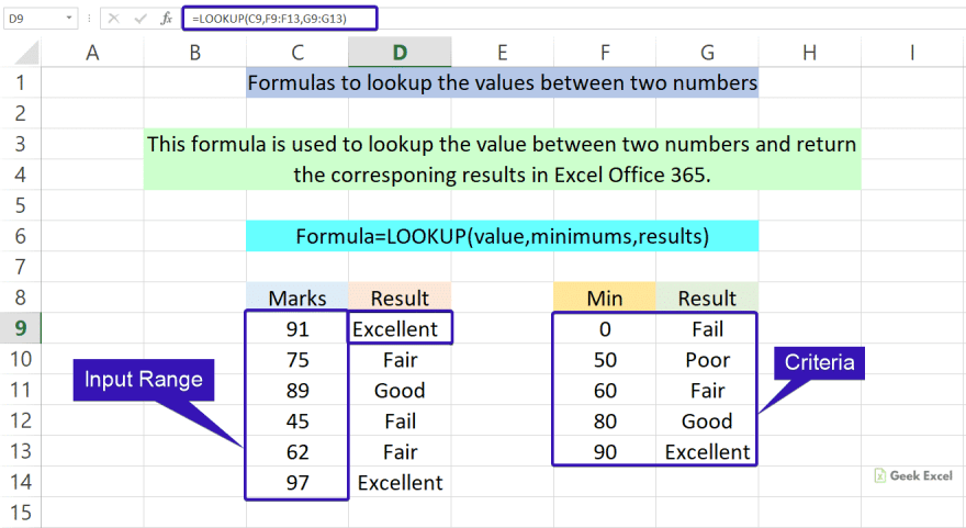
Let’s see how to find the value between two numbers.
- First, we will give the input Marks in Column B.

- We have assigned the criteria between the two values in Column E and Column F.

- Now, we want to find the result based on the input marks.
- So, enter the given formula in Cell C3, you can also see the formula in the formula bar section.

- Finally, click the ENTER key to get the results.

Wind-Up:
From this short tutorial, we have described the simple formula used to lookup the values between two numbers in Excel. Make use of it. Please state your queries in the below comment section let me know. We will assist you. To learn more, check out Geek Excel!! *and Excel Formulas *!!


Top comments (0)