Excel Formulas to Lookup the Entire Column ~ Simple Guide!!

In the previous post, we talked that how to lookup value and then returns entire rows of a matched value in a range. Sometimes we need to lookup entire columns using some key or lookup value in Excel. In that case, you may use the traditional HLOOKUP formula. But we can retrieve the entire column in one hit using INDEX-MATCH. Let’s see how. Get an official version of ** MS Excel** from the following link: https://www.microsoft.com/en-in/microsoft-365/excel

General Formula:

• To look up the value from the entire column in Excel, you can use the below formula.

=INDEX(data,column_no,MATCH(value,headers,0))

Syntax Explanations:

• INDEX – The INDEX function returns the value at a given position in a range or array.
• MATCH – In Excel, this function will locate the position of a lookup value in a row, column, or table. Read more on the MATCH function.
• Comma symbol (,) – It is a separator that helps to separate a list of values.
• Parenthesis () – The main purpose of this symbol is to group the elements.
• Data – It represents the input ranges in your worksheet.
• Value – It is the criteria that want to get the values.
• Headers – It is the heading of the input data from your worksheet.

Example:

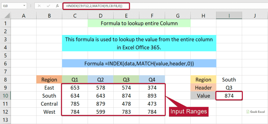
Let’s see how to find the value from the entire column based on certain criteria.

• First, we will give the input values from Column ** B** to Column F.

• Then, enter the given formula in the formula bar section or cell I10.

• Finally, we will get the result in the selected cell.

Wind-Up:

Hope you understood the simple and useful steps to lookup the value from the entire column in Excel. Make use of it. If you have any questions, feel free to comment. Click here to know more about Geek Excel!! And Excel Formulas!!

Related Articles:

• Excel Formulas to Lookup the Values between Two Numbers!!
• Excel Formulas to Lookup and Sum Column ~ With Clear-Cut Example!!