We have already learned how to convert the date into text format in Excel. Similarly, here we will show the simple formulas used to convert the text into date format in Excel. Let’s step into this article!! Get an official version of ** MS Excel** from the following link: https://www.microsoft.com/en-in/microsoft-365/excel
General Formula:
- You can use the below formula to convert the calendar date into text format.
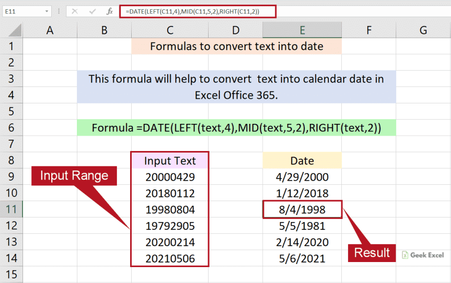
*=DATE(LEFT(text,4),MID(text,5,2),RIGHT(text,2)) *
Syntax Explanations:
- DATE – In Excel, the DATE function will combine three different values and returns them as a date.
- RIGHT – This function helps to extract the characters from the right side of a text string. Read more on the RIGHT function.
- MID – The Excel MID function is used to extract the number (starting from the left side) or characters from the given string.
- LEFT – It will extract the first character (starting from the left side) or characters from the given string based on the number you specified. Read more on the LEFT function.
- Text – It represents the input text on your worksheet.
- Comma symbol (,) – It is a separator that helps to separate a list of values.
- Parenthesis () – The main purpose of this symbol is to group the elements.
Practical Example:
Let’s consider the below example image.
- First, we will enter the input values in Column B.
- Now we are going to convert them into normal date format.

- So, apply the above-given formula to the formula bar section and press the ENTER key.

- Finally, we will get the result in the selected cell.

Bottom-Line:
Hope you like this article on how to convert the text into the date format in Excel. Let me know if you have any doubts regarding this article or any other article on this site.
Thank you so much for visiting *Geek Excel!! **If you want to learn more helpful formulas, check out Excel Formulas *!! **


Top comments (0)