If you've been following along with the series so far, you should be familiar with the overall concept of Big O notation, as well as being able to recognize constant, linear, logarithmic and polynomial time complexities.

For this last entry, we'll wrap up with some of the less common "common complexities", and a little bit about space complexity.

O(2^n) Exponential Time

While O(n^2) is sometimes mistakenly referred to as exponential time (it's actually called polynomial time), true exponential time is another thing entirely. Exponential time refers to functions that grow at a rate of O(2^n).

This is actually much more complex than polynomial time, and can result in unacceptably long runtimes. For every single increase in input size, the entire number of operations doubles!

At input size 1, number of operations is 2.
At input size 2, number of operations is 4.
At input size 10, number of operations is 1,024.
At input size 11, number of operations is 2,048!

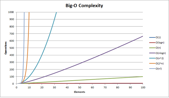
Here is a direct comparison to the other common complexities we've gone over:

n = 11

Constant time/O(1): 1 operation
Logarithmic time/O(log n): around 4 operations
Linear time/O(n): 11 operations
Polynomial time/O(n^2): 121 operations

Exponential time/O(2^n): 2,048 operations

As you can see, things can get out of hand very quickly.

Some kinds of recursion can lead to algorithms with O(2^n) time complexity, so it's worth watching out for. But, if you're using the proper data structures and techniques, exponential time algorithms should be avoidable or optimizable to a more efficient solution.

O(n!) Factorial Time

Now if you thought O(2^n) was bad, you don't want to know about O(n!).

Thinking through factorial time, we can see that increasing the input by 1, doesn't just double the number of operations, it multiplies them by whatever our new value is. In other words, the 11th input, will take 11 times as many operations as the 10th.

Let's look at some sample values like before:

At input size 1, number of operations is 1. (not bad)
At input size 2, number of operations is 2. (wait this is actually less)
At input size 3, number of operations is 6. (hmmmmm )
At input size 4, number of operations is 24. (that's a pretty big jump)
At input size 10, number of operations is 3,628,800. (pretty wild)
At input size 11, number of operations is 39,916,800!

Obviously, algorithms in factorial time quickly become too complex to be very useful. However, there is a famous example of a factorial algorithm called "the travelling salesman" which shows at least one use case. It's pretty interesting, and you can go really deep into computational complexity, if you're up for it.

Space Complexity

So far, for this whole series, we've only been talking about Big-O notation in regards to time complexity.

But, as you probably already know, there is another aspect to algorithms called space complexity. Space complexity is also expressed using big-o, and goes hand in hand with time complexity. In fact, you already know everything you need to understand space complexity. All we have to do is change our perspective a bit.

Space complexity describes how much more space in memory an algorithm uses as the input size increases.

Pretty familiar, right. All we need to do is look at memory use instead of number of operations. In other words, instead of focusing on what we "do", we'll look at what we "make".

Take, for example, a basic factorial method

def factorial(n)
   if n < 1
      return 0
   elsif n == 1
      return 1
   else
      return n * factorial(n-1)
   end
end

We can calculate that our time complexity is O(n). The conditional will be constant time, but since we will have to call our function recursively on all numbers up to n, we can see that it runs in linear time.

Now let's look at the space complexity. To do this, we'll change our perspective from "do" to "make".

Is there any place in our code where we create a new value? Yes, There is. When we do our recursive call we need to make the value "n - 1". This will require a new space to record the value of "n-1". So, we can say that as our n increases the amount of space it requires will increase.

In this case, an input of 10 will make 10 new values, and an input of 100 will make 100 new values (0-99). If we apply our big-O notation logic, it's easy to see that the space complexity will be O(n), or linear space complexity.

Just remember that space complexity follows the same logic, we're just applying it to a different aspect of the algorithm.

Conclusion

If you've followed through from the beginning, hopefully you now know enough about big-o notation and complexity theory to confidently identify common complexities. If not, I hope that I at least encouraged you to investigate further and gave a decent enough intro to the subject.