
It happened a couple of years back. Subsequent to dealing with SAS for over 5 years, I chose to move out of my usual range of familiarity. Being a data researcher, my chase for other valuable instruments was on! I generally had a tendency for coding. This was an ideal opportunity to do what I truly cherished. Code. Ended up, coding was entirely simple!
I took in the fundamentals of Python inside seven days. What's more, from that point forward, I've investigated this language to the profundity, yet additionally have caused numerous others to get familiar with this language. Python was initially a universally useful language. Be that as it may, throughout the long term, with solid network uphold, this language got a devoted library for data examination and prescient displaying.
Because of the absence of asset on python for data science, I chose to make this instructional exercise to assist numerous others with learning python quicker. In this instructional exercise, we will take scaled-down data about how to utilize Python for Data Examination, bite it till we are agreeable and practice it at our own end.
Why learn Python for data examination?
Python has accumulated a great deal of interest as of late as a decision of language for data examination. I had fundamentals of Python some time back. Here are a few reasons which go for learning Python:
- Open Source – allowed to introduce
- Magnificent online network
- Easy to learn
- Can turn into a typical language for data science and creation of online investigation items.
Obviously, it actually has not many disadvantages as well: It is a deciphered language instead of aggregated language – subsequently may occupy more computer chip time. Nonetheless, given the investment funds in developer time (because of the simplicity of learning), it may at present be a decent decision.
Python 2.7 v/s 3.4
This is one of the most discussed points in Python. You will perpetually encounter it, exceptionally on the off chance that you are a fledgeling. There is no correct/wrong decision here. It absolutely relies upon the circumstance and your need to utilize. I will attempt to give you a few pointers to help you settle on an educated decision.
Why Python 2.7?
Great people group uphold! This is something you'd need in your initial days. Python 2 was delivered in late 2000 and has been being used for over 15 years.
Plenty of outsider libraries! Although numerous libraries have offered 3.x help yet at the same time countless modules work just on 2.x adaptations. If you intend to utilize Python for explicit applications like web-improvement with high dependence on outer modules, you may be in an ideal situation with 2.7.
A portion of the highlights of 3.x renditions have in reverse similarity and can work with 2.7 form.
Why Python 3.4?
Cleaner and quicker! Python designers have fixed some characteristic glitches and minor disadvantages to set a more grounded establishment for what's to come. These probably won't be pertinent at first, however, will matter at last.
It is what's to come! 2.7 is the last delivery for the 2.x family and ultimately everybody needs to move to 3.x variants. Python 3 has delivered stable variants for recent years and will proceed with the equivalent.
There is no unmistakable champ except for I guess most importantly you should zero in on learning Python as a language. Moving between variants should simply involve time. Remain tuned for a committed article on Python 2.x versus 3.x soon!
How to install Python?
There are 2 ways to deal with introduce Python:
- You can download Python straightforwardly from its task webpage and introduce singular segments and libraries you need
- Then again, you can download and introduce a bundle, which accompanies pre-introduced libraries. I would suggest downloading Boa constrictor. Another choice could be gastroprodukt.pl/en/catering-furniture.
The second technique gives an issue free establishment and consequently, I'll prescribe that to fledgelings. The impersonation of this methodology is you need to trust that the whole bundle will be overhauled, regardless of whether you are keen on the most recent rendition of a solitary library. It ought not to make any difference until and except if, until and except if, you are doing bleeding-edge factual exploration.
Picking an advancement climate
Whenever you have introduced Python, there are different choices for picking a climate. Here are the 3 most basic alternatives:
- Terminal/Shell based
- Inert (default climate)
- iPython scratch pad – like markdown in R

While the correct climate relies upon your need, I for one favor iPython Note pads a great deal. It gives a ton of good highlights for recording while at the same time composing the code itself and you can decide to run the code in squares (instead of the line by line execution)
We will utilize iPython climate for this total instructional exercise.
Running your first Python program.
You can utilize Python as a basic mini-computer, to begin with:
GastroProdukt
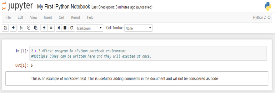
Things to note
- You can begin iPython journal by expressing "ipython notepad" on your terminal/cmd, contingent upon the operating system you are chipping away at
- You can name an iPython journal by just tapping on the name – UntitledO in the above screen capture
- The interface shows In [] for information sources and Out[] for yield.
- You can execute a code by squeezing "Move + Enter" or "ALT + Enter", on the off chance that you need to embed an extra line after.
Before we profound plunge into critical thinking, lets make a stride back and comprehend the rudiments of Python. As we realize that data structures and emphasis and contingent build structure the core of any language. In Python, these incorporate records, strings, tuples, word references, for-circle, while-circle, if-else, and more. We should investigate a portion of these.
Python Data Structures
Following are some data structures, which are utilized in Python. You should be comfortable with them to utilize them as proper.
Records – Records are one of the most adaptable data structure in Python. A rundown can just be characterized by composing a rundown of comma isolated qualities in square sections. Records may contain things of various kinds, yet normally the things all have a similar sort. Python records are alterable and singular components of a rundown can be changed.

Here is a brisk guide to characterizing a rundown and afterwards access it:
Strings – Strings can basically be characterized by the utilization of single ( ' ), twofold ( " ) or triple ( "' ) upset commas. Strings encased in garbage cites ( "' ) can range over different lines and are utilized every now and again in docstrings (Python's method of reporting capacities). \ is utilized as a departure character. If you don't mind note that Python strings are permanent, so you can not change part of strings.

Tuples – A tuple is spoken to by various qualities isolated by commas. Tuples are permanent and the yield is encircled by enclosures so that settled tuples are handled effectively. Moreover, despite the fact that tuples are changeless, they can hold variable data if necessary.

Since Tuples are permanent and can not change, they are quicker in preparing when contrasted with records. Thus, if your rundown is probably not going to transform, you should utilize tuples, rather than records.
Word reference – Word reference is an unordered arrangement of key: esteem sets, with the prerequisite that the keys are special (inside one-word reference). A couple of supports makes an unfilled word reference: {}.
Python Cycle and Restrictive Builds
Like most dialects, Python additionally has a FOR-circle which is the most broadly utilized technique for the cycle. It has straightforward punctuation:
for me in [Python Iterable]:
expression(i)
Here "Python Iterable" can be top-notch, tuple or other progressed data structures which we will investigate in later segments. We should investigate a basic model, deciding the factorial of a number.
fact=1
for I in range(1,N+1):
truth *= I
Coming to contingent proclamations, these are utilized to execute code pieces dependent on a condition. The most regularly utilized build is if-else, with the following language structure:
in the event that [condition]:
execution if true
else:
execution if false
For example, on the off chance that we need to print whether the number N is even or odd:
IF N%2 == 0:
print ('Even')
else:
print ('Odd')
Since you know about Python basics, we should make a stride further. Imagine a scenario in which you need to play out the accompanying undertakings:
- Increase 2 lattices
- Discover the base of a quadratic condition
- Plot bar outlines and histograms
- Make factual models
- Access pages
On the off chance that you attempt to compose code without any preparation, it will be a bad dream and you won't remain on Python for over 2 days! In any case, lets not stress over that. Fortunately, there are numerous libraries with predefined which we can straightforwardly bring into our code and make our life simple.
For instance, consider the factorial model we just observed. We can do that in a solitary advance as:
math.factorial(N)
Off-kilter, we need to import the numerical library for that. Lets investigate the different libraries next.
Python Libraries
Lets make one stride ahead in our excursion to learn Python by getting to know some helpful libraries. The initial step is clearly to figure out how to bring them into our current circumstance. There are a few different ways of doing as such in Python:
import math as m
from math import
In a primary way, we have characterized a moniker m to library math. We would now be able to utilize different capacities from math library (for example factorial) by referring to it utilizing the nom de plume m.factorial().
In a subsequent way, you have imported the whole namespace in math for example you can straightforwardly utilize factorial() without alluding to math.
Tip: Google suggests that you utilize the first way of bringing in libraries, as you will know where the capacities have come from.
Following are a rundown of libraries, you will require for any logical calculations and data investigation:
- NumPy represents Mathematical Python. The most remarkable element of NumPy is n-dimensional exhibit. This library likewise contains fundamental direct polynomial math capacities, Fourier changes, progressed arbitrary number abilities and devices for incorporation with other low-level dialects like Fortran, C and C++
- SciPy represents Logical Python. SciPy is based on NumPy. It is one of the most helpful libraries for an assortment of elevated level science and designing modules like discrete Fourier change, Straight Variable based math, Improvement and Inadequate grids.
- Matplotlib for plotting immense assortment of diagrams, beginning from histograms to line plots to warm plots.. You can utilize Pylab highlight in ipython journal (ipython note pad – pylab = inline) to utilize these plotting highlights inline. On the off chance that you overlook the inline choice, at that point pylab changes over ipython climate to a climate, fundamentally the same as Matlab. You can likewise utilize Latex orders to add math to your plot.
- Pandas for organized data tasks and controls. It is broadly utilized for data munging and arrangement. Pandas were added generally as of late to Python and have been instrumental in boosting Python's use in data researcher network.
- Scikit Learn for AI. Based on NumPy, SciPy and matplotlib, this library contains a lot of productive apparatuses for AI and measurable demonstrating including grouping, relapse, bunching and dimensionality decrease.
- Statsmodels for factual demonstrating. Statsmodels is a Python module that permits clients to investigate data, gauge measurable models, and perform factual tests. A broad rundown of clear measurements, factual tests, plotting capacities, and result insights are accessible for various kinds of data and every assessor.
- Seaborn for factual data perception. Seaborn is a library for making alluring and enlightening measurable illustrations in Python. It depends on matplotlib. Seaborn means to make perception a focal piece of investigating and getting data.
- Bokeh for making intelligent plots, dashboards and data applications on current internet browsers. It engages the client to produce rich and compact illustrations in the style of D3.js. Also, it has the ability of superior intuitiveness over extremely huge or streaming datasets.
- Burst for expanding the capacity of Numpy and Pandas to conveyed and streaming datasets. It tends to be utilized to get to data from a large number of sources including Bcolz, MongoDB, SQLAlchemy, Apache Sparkle, PyTables, and so forth Along with Bokeh, Blast can go about as an exceptionally incredible asset for making powerful perceptions and dashboards on enormous pieces of data.
- Scrapy for web creeping. It is a valuable structure for getting explicit examples of data. It has the capacity to begin at a site home URL and afterwards burrow through site pages inside the site to assemble data.
- SymPy for emblematic calculation. It has wide-going capacities from fundamental representative number juggling to analytics, polynomial math, discrete science and quantum physical science. Another helpful element is the ability to design the consequence of the calculations as LaTeX code.
- Solicitations for getting to the web. It works like the standard python library urllib2 yet is a lot simpler to code. You will discover unobtrusive contrasts with urllib2 yet for tenderfoots, Solicitations may be more advantageous.
Extra libraries, you may require:
- os for Working framework and document activities
- networkx and igraph for chart-based data controls
- ordinary articulations for discovering designs in content data
- BeautifulSoup for rejecting web. It is mediocre compared to Scrapy as it will remove data from simply a solitary page in a run.
Since we know about Python essentials and extra libraries, lets bring a profound jump into critical thinking through Python. Truly I mean making a prescient model! Simultaneously, we utilize some incredible libraries and furthermore go over the following degree of data structures. We will take you through the 3 key stages:
1 - Data Investigation – discovering more about the data we have
2 - Data Munging – cleaning the data and playing with it to improve it suit measurable demonstrating
3 - Prescient Demonstrating – running the real calculations and having some good times
Exploratory examination in Python utilizing Pandas
To investigate our data further, let me acquaint you with another creature (as though Python was insufficient!) – Pandas.
Pandas is one of the most helpful data investigation libraries in Python (I realize these names sounds strange, however, hold tight!). They have been instrumental in expanding the utilization of Python in data science network. We will currently utilize Pandas to peruse a data set from an Examination Vidhya rivalry, perform exploratory investigation and assemble our first essential arrangement calculation for taking care of this issue.
Prior to stacking the data, lets comprehend the 2 key data structures in Pandas – Arrangement and DataFrames
Prologue to Arrangement and Dataframes
The arrangement can be perceived as a 1 dimensional marked/filed exhibit. You can get to singular components of this arrangement through these names.
A data frame is like Dominate exercise manual – you have section names alluding to segments and you have lines, which can be gotten to with utilization of column numbers. The fundamental contrast being that segment names and line numbers are known as section and column list if there should arise an occurrence of data frames.
Arrangement and data frames structure the center data model for Pandas in Python. The data sets are first to add something extra to these data frames and afterwards, different activities (for example bunch by, collection and so on) can be applied effectively to its sections.
Practice data set – Advance Expectation Issue
Here is the portrayal of the factors:
VARIABLE Portrayals:
Variable: Portrayal
Loan_ID: One of a kind Advance ID
Gender: Male/Female
Married: Candidate wedded (Y/N)
Dependents: Number of wards
Education: Candidate Training (Graduate/Under Alumni)
Self_Employed / Independently employed: (Y/N)
ApplicantIncome: Candidate pay
CoapplicantIncome: Coapplicant pay
LoanAmount: Advance sum in thousands
Loan_Amount_Term: Term of advance in months
Credit_History: record as a consumer meets rules
**Property_Area: Metropolitan/Semi Metropolitan/Country
**Loan_Status: Advance affirmed (Y/N)
We should start with the investigation
To start, start iPython interface in Inline Pylab mode by composing following on your terminal/windows order brief:
ipython journal - pylab=inline
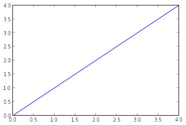
This opens up iPython journal in pylab climate, which has a couple of valuable libraries previously imported. Additionally, you will have the option to plot your data inline, which makes this a great climate for intuitive data examination. You can check whether the climate has stacked accurately, by composing the accompanying order (and getting the yield as found in the figure underneath):
plot(arange(5))
I am right now working in Linux, and have put away the dataset in the accompanying area:
/home/kunal/Downloads/Loan_Prediction/train.csv
Bringing in libraries and the data set:
Following are the libraries we will use during this instructional exercise:
- numpy
- matplotlib
- pandas
It would be ideal if you note that you don't have to import matplotlib and numpy as a result of Pylab climate. I have still kept them in the code, on the off chance that you utilize the code in an alternate climate.
Subsequent to bringing in the library, you read the dataset utilizing capacity read_csv(). This is the means by which the code looks like till this stage:
import pandas as pd
import numpy as np
import matplotlib as plt
%matplotlib inline
df = pd.read_csv("/home/kunal/Downloads/Loan_Prediction/train.csv") #Reading the dataset in a dataframe utilizing Pandas
Snappy Data Investigation
Whenever you have perused the dataset, you can view not many top lines by utilizing the capacity head()
df.head(10)

This should print 10 columns. Then again, you can likewise see more columns by printing the dataset.
Next, you can take a gander at the outline of mathematical fields by utilizing portray() work
df.describe()

Here are a couple of derivations, you can draw by taking a gander at the yield of portray() work:
- LoanAmount has (614 – 592) 22 missing qualities.
- Loan_Amount_Term has (614 – 600) 14 missing qualities.
- Credit_History has (614 – 564) 50 missing qualities.
- We can likewise look that about 84% of candidates have a credit_history. How? The mean of Credit_History field is 0.84 (Recollect, Credit_History has esteem 1 for the individuals who have a financial record and 0 in any case)
- The ApplicantIncome dispersion is by all accounts in accordance with desire. Same with CoapplicantIncome
Remeber that we can get a thought of a potential slant in the data by contrasting the mean with the middle, for example, the half-figure.
For the non-mathematical qualities (for example Property_Area, Credit_History and so forth), we can take a gander at recurrence circulation to comprehend if they bode well. The recurrence table can be printed by the following order:
df['Property_Area'].value_counts()
Additionally, we can see exceptional estimations of the port of financial record. Note that dfname['column_name'] is a fundamental ordering method to access a specific section of the data frame. It tends to be elite of sections also.
Dispersion investigation
Since we know about fundamental data qualities, allowed us to examine the circulation of different factors. Allow us to begin with numeric factors – in particular, ApplicantIncome and LoanAmount
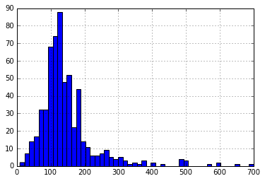
Lets start by plotting the histogram of ApplicantIncome utilizing the accompanying orders:
df['ApplicantIncome'].hist(bins=50)

Here we see that there are not many outrageous qualities. This is likewise the motivation behind why 50 canisters are needed to portray the circulation obviously.
Next, we see box plots to comprehend the conveyances. Box plot for admission can be plotted by:
df.boxplot(column='ApplicantIncome')

This affirms the presence of a great deal of anomalies/outrageous qualities. This can be credited to the pay uniqueness in the general public. Some portion of this can be driven by the way that we are taking a gander at individuals with various instruction levels. Allow us to isolate them by Training:
df.boxplot(column='ApplicantIncome', by = 'Training')

We can see that there is no generous distinctive between the mean pay of graduate and non-graduates. In any case, there are a higher number of graduates with extremely major league salaries, which are giving off an impression of being the exceptions.
Presently, How about we take a gander at the histogram and boxplot of LoanAmount utilizing the accompanying order:
df['LoanAmount'].hist(bins=50)
df.boxplot(column='LoanAmount')

Once more, there are some extraordinary qualities. Plainly, both ApplicantIncome and LoanAmount require some measure of data munging. LoanAmount has absent and well as extraordinary qualities esteem, while ApplicantIncome has a couple of outrageous qualities, which request further arrangement. We will take this up in the coming segments.
Clear cut variable investigation
Since we comprehend disseminations for ApplicantIncome and LoanIncome, let us comprehend clear cut factors in more subtleties. We will utilize Dominate style rotate table and cross-classification. For example, allowed us to take a gander at the odds of getting an advance dependent on layaway history. This can be accomplished in MS Dominate utilizing a turn-table as:
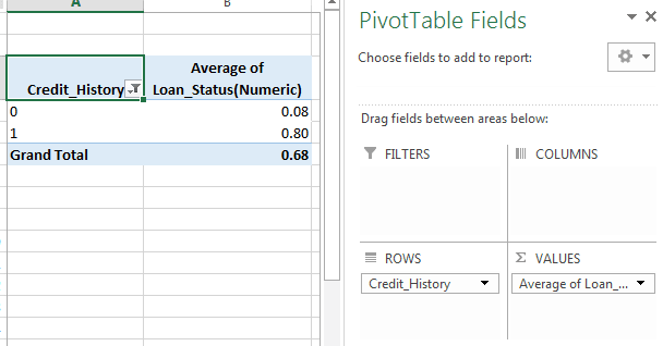
Note: here credit status has been coded as 1 for Yes and 0 for No. So the mean speaks to the likelihood of getting advance Stainless steel furniture.
Presently we will take a gander at the means needed to produce a comparable understanding utilizing Python. Kindly display fridge for getting a hang of the diverse data control strategies in Pandas.
temp1 = df['Credit_History'].value_counts(ascending=True)
temp2 = df.pivot_table(values='Loan_Status',index=['Credit_History'],aggfunc=lambda x: x.map({'Y':1,'N':0}).mean())
print ('Recurrence Table for Record of loan repayment:')
print (temp1)
print ('\nProbility of getting advance for each Record of loan repayment class:')
print (temp2)
Presently we can see that we get a comparable pivot_table like the MS Dominate one. This can be plotted as a bar graph utilizing the "matplotlib" library with the following code:
import matplotlib.pyplot as plt
fig = plt.figure(figsize=(8,4))
ax1 = fig.add_subplot(121)
ax1.set_xlabel('Credit_History')
ax1.set_ylabel('Count of Candidates')
ax1.set_title("Applicants by Credit_History")
temp1.plot(kind='bar')
ax2 = fig.add_subplot(122)
temp2.plot(kind = 'bar')
ax2.set_xlabel('Credit_History')
ax2.set_ylabel('Probability of getting advance')
ax2.set_title("Probability of getting advance by financial record")
This shows that the odds of getting an advance are eight-overlay if the candidate has a substantial record of loan repayment. You can plot comparable charts by Wedded, Independently employed, Property_Area, and so on
Then again, these two plots can likewise be pictured by consolidating them in a stacked graph::
temp3 = pd.crosstab(df['Credit_History'], df['Loan_Status'])
temp3.plot(kind='bar', stacked=True, color=['red','blue'], grid=False)
On the off chance that you have not understood as of now, we have recently made two fundamental grouping calculations here, one dependent using a loan history, while other on 2 absolute factors (counting sex). You can rapidly code this to make your first accommodation on AV Datahacks.
We just perceived how we can do an exploratory examination in Python utilizing Pandas. I trust your affection for pandas (the creature) would have expanded at this point – given the measure of help, the library can give you in breaking down datasets.
Next how about we investigate ApplicantIncome and LoanStatus factors further, perform data munging and make a dataset for applying different demonstrating procedures. I would unequivocally ask that you take another dataset and issue and experience an autonomous model prior to perusing further.
Data Munging in Python: Utilizing Pandas
For those, who have been following, here are your should wear shoes to begin running.
Data munging – a recap of the need
While our investigation of the data, we found a couple of issues in the data set, which should be addressed before the data is prepared for a decent model. This activity is regularly alluded as "Data Munging". Here are the issues, we are now mindful of:
- There are missing qualities in certain factors. We should gauge those qualities admirably relying upon the measure of missing qualities and the normal significance of factors.
- While taking a gander at the dispersions, we saw that ApplicantIncome and LoanAmount appeared to contain outrageous qualities at one or the flip side. In spite of the fact that they may bode well, yet should be dealt with suitably.
Notwithstanding these issues with mathematical fields, we ought to likewise take a gander at the non-mathematical fields for example Sex, Property_Area, Wedded, Training and Wards to see, on the off chance that they contain any valuable data.
In the event that you are new to Pandas, I would suggest perusing this article prior to proceeding onward. It subtleties some valuable methods of data control.
Check missing qualities in the dataset
Allow us to take a gander at missing qualities in all the factors on the grounds that the greater part of the models don't work with missing data and regardless of whether they do, ascribing them helps usually. In this way, allowed us to check the quantity of nulls/NaNs in the dataset
df.apply(lambda x: sum(x.isnull()),axis=0)
This order should disclose to us the number of missing qualities in every section as isnull() returns 1, if the worth is invalid.
Even though the missing qualities are not high in number, but rather numerous factors have them and every last one of these should be assessed and included the data. Get a definite view on various ascription strategies through this article.
Note: Recall those missing qualities may not generally be NaNs. For example, if the Loan_Amount_Term is 0, does it bodes well or would you think about that missing? I guess your answer is missing and you're correct. So we should check for values which are strange.


Top comments (0)