
Ahana provides managed Presto clusters running in your AWS account.
Presto is an open-source distributed SQL query engine, originally developed at Facebook, now hosted under the Linux Foundation. It connects to multiple databases or other data sources (for example, Amazon S3). We can use a Presto cluster as a single compute engine for an entire data lake.
Presto implements the data federation feature: you can process data from multiple sources as if they were stored in a single database. Because of that, you don’t need a separate ETL (Extract-Transform-Load) pipeline to prepare the data before using it. However, running and configuring a single-point-of-access for multiple databases (or file systems) requires Ops skills and an additional effort.
However, no data engineer wants to do the Ops work. Using Ahana, you can deploy a Presto cluster within minutes without spending hours configuring the service, VPCs, and AWS access rights. Ahana hides the burden of infrastructure management and allows you to focus on processing your data.
What is Cube?
Cube is a headless BI platform for accessing, organizing, and delivering data. Cube connects to many data warehouses, databases, or query engines, including Presto, and allows you to quickly build data applications or analyze your data in BI tools. It serves as the single source of truth for your business metrics.

This article will demonstrate the caching functionality, access control, and flexibility of the data retrieval API.
Integration
Cube's battle-tested Presto driver provides the out-of-the-box connectivity to Ahana.
You just need to provide the credentials: Presto host name and port, user name and password, Presto catalog and schema. You'll also need to set CUBEJS_DB_SSL to true since Ahana has secures Presto connections with SSL.
Check the docs to learn more about connecting Cube to Ahana.
Example: Parsing logs from multiple data sources with Ahana and Cube
Let's build a real-world data application with Ahana and Cube.
We will use Ahana to join Amazon Sagemaker Endpoint logs stored as JSON files in S3 with the data retrieved from a PostgreSQL database.
Suppose you work at a software house specializing in training ML models for your clients and delivering ML inference as a REST API. You have just trained new versions of all models, and you would like to demonstrate the improvements to the clients.
Because of that, you do a canary deployment of the versions and gather the predictions from the new and the old models using the built-in logging functionality of AWS Sagemaker Endpoints: a managed deployment environment for machine learning models. Additionally, you also track the actual production values provided by your clients.
You need all of that to prepare personalized dashboards showing the results of your hard work.
Let us show you how Ahana and Cube work together to help you achieve your goal quickly without spending days reading cryptic documentation.
You will retrieve the prediction logs from an S3 bucket and merge them with the actual values stored in a PostgreSQL database. After that, you calculate the ML performance metrics, implement access control, and hide the data source complexity behind an easy-to-use REST API.

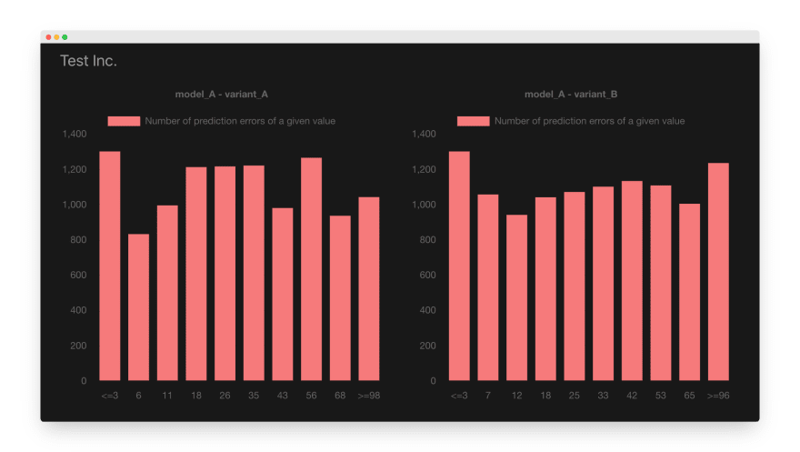
In the end, you want a dashboard looking like this:

How to configure Ahana?
Allowing Ahana to access your AWS account
First, let’s login to Ahana, and connect it to your AWS account. We must create an IAM role allowing Ahana to access our AWS account.
On the setup page, click the “Open CloudFormation” button. After clicking the button, we get redirected to the AWS page for creating a new CloudFormation stack from a template provided by Ahana. Create the stack and wait until CloudFormation finishes the setup.
When the IAM role is configured, click the stack’s Outputs tab and copy the AhanaCloudProvisioningRole key value.

We have to paste it into the Role ARN field on the Ahana setup page and click the “Complete Setup” button.

Creating an Ahana cluster
After configuring AWS access, we have to start a new Ahana cluster.
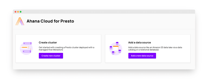
In the Ahana dashboard, click the “Create new cluster” button.
In the setup window, we can configure the type of the AWS EC2 instances used by the cluster, scaling strategy, and the Hive Metastore. If you need a detailed description of the configuration options, look at the “Create new cluster” section of the Ahana documentation.

Remember to add at least one user to your cluster! When we are satisfied with the configuration, we can click the “Create cluster” button. Ahana needs around 20-30 minutes to setup a new cluster.
Retrieving data from S3 and PostgreSQL
After deploying a Presto cluster, we have to connect our data sources to the cluster because, in this example, the Sagemaker Endpoint logs are stored in S3 and PostgreSQL.
Adding a PostgreSQL database to Ahana
In the Ahana dashboard, click the “Add new data source” button. We will see a page showing all supported data sources. Let’s click the “Amazon RDS for PostgreSQL” option.
In the setup form displayed below, we have to provide the database configuration and click the “Add data source” button.

Adding an S3 bucket to Ahana
AWS Sagemaker Endpoint stores their logs in an S3 bucket as JSON files. To access those files in Presto, we need to configure the AWS Glue data catalog and add the data catalog to the Ahana cluster.
We have to login to the AWS console, open the AWS Glue page and add a new database to the data catalog (or use an existing one).

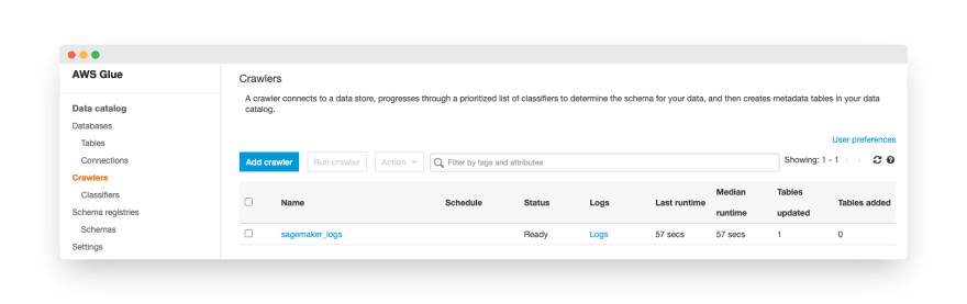
Now, let’s add a new table. We won’t configure it manually. Instead, let’s create a Glue crawler to generate the table definition automatically. On the AWS Glue page, we have to click the “Crawlers” link and click the “Add crawler” button.
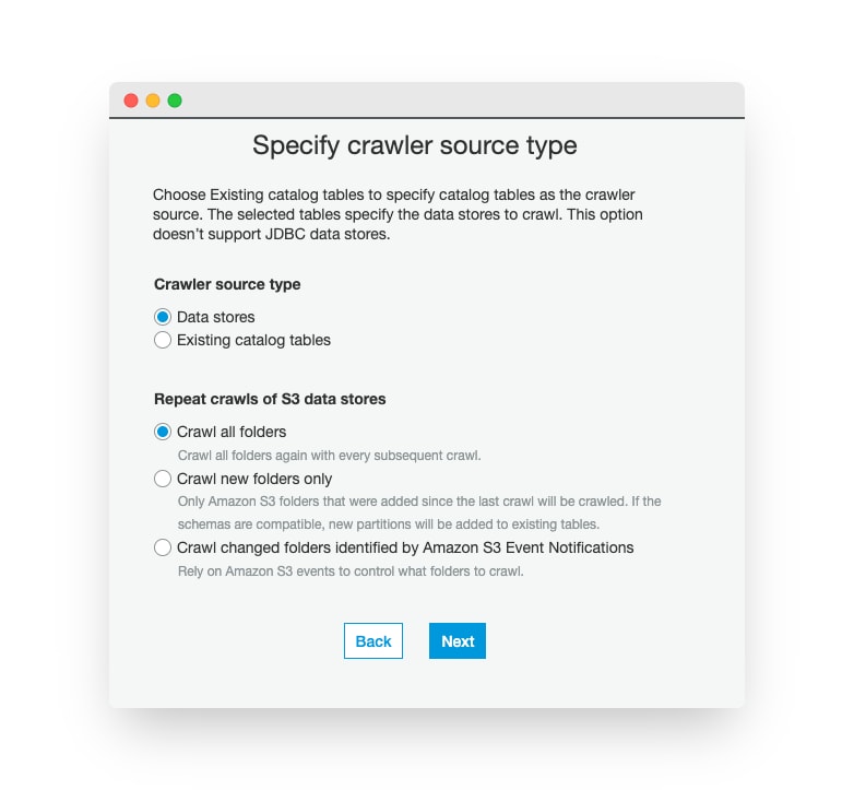
After typing the crawler’s name and clicking the “Next” button, we will see the Source Type page. On this page, we have to choose the “Data stores” and “Crawl all folders” (in our case, “Crawl new folders only” would work too).
On the “Data store” page, we pick the S3 data store, select the S3 connection (or click the “Add connection” button if we don’t have an S3 connection configured yet), and specify the S3 path.
Note that Sagemaker Endpoints store logs in subkeys using the following key structure: endpoint-name/model-variant/year/month/day/hour. We want to use those parts of the key as table partitions.
Because of that, if our Sagemaker logs have an S3 key: s3://the_bucket_name/sagemaker/logs/endpoint-name/model-variant-name/year/month/day/hour, we put only the s3://the_bucket_name/sagemaker/logs key prefix in the setup window!

Let’s click the “Next” button. In the subsequent window, we choose “No” when asked whether we want to configure another data source. Glue setup will ask about the name of the crawler’s IAM role. We can create a new one:

Next, we configure the crawler’s schedule. A Sagemaker Endpoint adds new log files in near real-time. Because of that, it makes sense to scan the files and add new partitions every hour:

In the output configuration, we need to customize the settings.
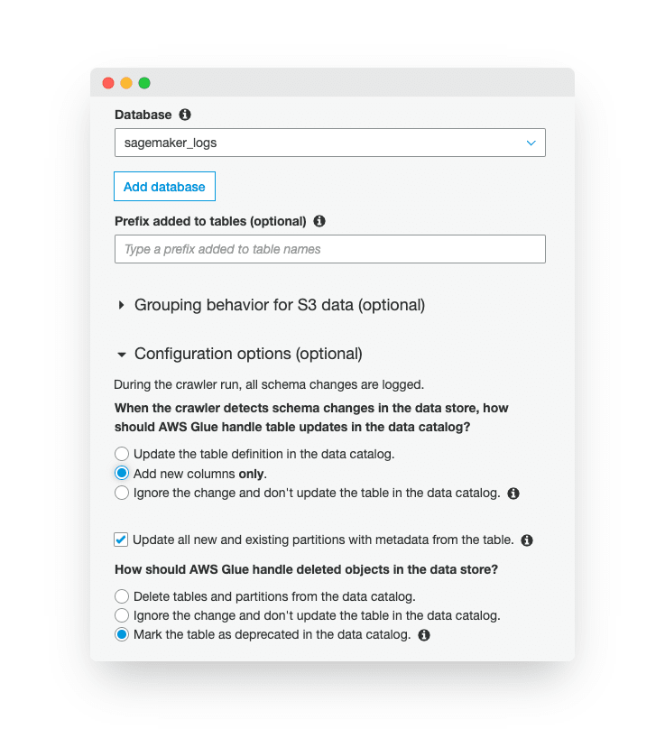
First, let’s select the Glue database where the new tables get stored. After that, we modify the “Configuration options.”
We pick the “Add new columns only” because we will make manual changes in the table definition, and we don’t want the crawler to overwrite them. Also, we want to add new partitions to the table, so we check the “Update all new and existing partitions with metadata from the table.” box.
Let’s click “Next.” We can check the configuration one more time in the review window and click the “Finish” button.
Now, we can wait until the crawler runs or open the AWS Glue Crawlers view and trigger the run manually. When the crawler finishes running, we go to the Tables view in AWS Glue and click the table name.
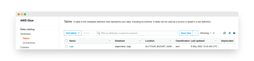
In the table view, we click the “Edit table” button and change the “Serde serialization lib” to “org.apache.hive.hcatalog.data.JsonSerDe” because the AWS JSON serialization library isn’t available in the Ahana Presto cluster.

We should also click the “Edit schema” button and change the default partition names to values shown in the screenshot below:

After saving the changes, we can add the Glue data catalog to our Ahana Presto cluster.
Configuring data sources in the Presto cluster
Go back to the Ahana dashboard and click the “Add data source” button. Select the “AWS Glue Data Catalog for Amazon S3” option in the setup form.

Let’s select our AWS region and put the AWS account id in the “Glue Data Catalog ID” field. After that, we click the “Open CloudFormation” button and apply the template. We will have to wait until CloudFormation creates the IAM role.
When the role is ready, we copy the role ARN from the Outputs tab and paste it into the “Glue/S3 Role ARN” field:

On the Ahana setup page, we click the “Add data source” button.
Adding data sources to an existing cluster
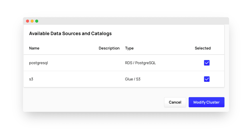
Finally, we can add both data sources to our Ahana cluster.
We have to open the Ahana “Clusters” page, click the “Manage” button, and scroll down to the “Data Sources” section. In this section, we click the “Manage data sources” button.
We will see another setup page where we check the boxes next to the data sources we want to configure and click the “Modify cluster” button. We will need to confirm that we want to restart the cluster to make the changes.
Writing the Presto queries
Before configuring Cube, let’s write the Presto queries to retrieve the data we want.
The actual structure of the input and output from an AWS Sagemaker Endpoint depends on us. We can send any JSON request and return a custom JSON object.
Let’s assume that our endpoint receives a request containing the input data for the machine learning model and a correlation id. We will need those ids to join the model predictions with the actual data.
Example input:
{"time_series": [51, 37, …, 7], "correlation_id": "cf8b7b9a-6b8a-45fe-9814-11a4b17c710a"}
In the response, the model returns a JSON object with a single “prediction” key and a decimal value:
{"prediction": 21.266147618448954}
A single request in Sagemaker Endpoint logs looks like this:
{"captureData": {"endpointInput": {"observedContentType": "application/json", "mode": "INPUT", "data": "eyJ0aW1lX3NlcmllcyI6IFs1MS40MjM5MjAzODYxNTAzODUsIDM3LjUwOTk2ODc2MTYwNzM0LCAzNi41NTk4MzI2OTQ0NjAwNTYsIDY0LjAyMTU3MzEyNjYyNDg0LCA2MC4zMjkwMzU2MDgyMjIwODUsIDIyLjk1MDg0MjgxNDg4MzExLCA0NC45MjQxNTU5MTE1MTQyOCwgMzkuMDM1NzA4Mjg4ODc2ODA1LCAyMC44NzQ0Njk2OTM0MzAxMTUsIDQ3Ljc4MzY3MDQ3MjI2MDI1NSwgMzcuNTgxMDYzNzUyNjY5NTE1LCA1OC4xMTc2MzQ5NjE5NDM4OCwgMzYuODgwNzExNTAyNDIxMywgMzkuNzE1Mjg4NTM5NzY5ODksIDUxLjkxMDYxODYyNzg0ODYyLCA0OS40Mzk4MjQwMTQ0NDM2OCwgNDIuODM5OTA5MDIxMDkwMzksIDI3LjYwOTU0MTY5MDYyNzkzLCAzOS44MDczNzU1NDQwODYyOCwgMzUuMTA2OTQ4MzI5NjQwOF0sICJjb3JyZWxhdGlvbl9pZCI6ICJjZjhiN2I5YS02YjhhLTQ1ZmUtOTgxNC0xMWE0YjE3YzcxMGEifQ==", "encoding": "BASE64"}, "endpointOutput": {"observedContentType": "application/json", "mode": "OUTPUT", "data": "eyJwcmVkaWN0aW9uIjogMjEuMjY2MTQ3NjE4NDQ4OTU0fQ==", "encoding": "BASE64"}}, "eventMetadata": {"eventId": "b409a948-fbc7-4fa6-8544-c7e85d1b7e21", "inferenceTime": "2022-05-06T10:23:19Z"}
AWS Sagemaker Endpoints encode the request and response using base64. Our query needs to decode the data before we can process it. Because of that, our Presto query starts with data decoding:
with sagemaker as (
  select
  model_name,
  variant_name,
  cast(json_extract(FROM_UTF8( from_base64(capturedata.endpointinput.data)), '$.correlation_id') as varchar) as correlation_id,
  cast(json_extract(FROM_UTF8( from_base64(capturedata.endpointoutput.data)), '$.prediction') as double) as prediction
  from s3.sagemaker_logs.logs
)
, actual as (
  select correlation_id, actual_value
  from postgresql.public.actual_values
)
After that, we join both data sources and calculate the absolute error value:
, logs as (
  select model_name, variant_name as model_variant, sagemaker.correlation_id, prediction, actual_value as actual
  from sagemaker
  left outer join actual
  on sagemaker.correlation_id = actual.correlation_id
)
, errors as (
  select abs(prediction - actual) as abs_err, model_name, model_variant from logs
),
Now, we need to calculate the percentiles using the approx_percentile function. Note that we group the percentiles by model name and model variant. Because of that, Presto will produce only a single row per every model-variant pair. That’ll be important when we write the second part of this query.
percentiles as (
  select approx_percentile(abs_err, 0.1) as perc_10,
  approx_percentile(abs_err, 0.2) as perc_20,
  approx_percentile(abs_err, 0.3) as perc_30,
  approx_percentile(abs_err, 0.4) as perc_40,
  approx_percentile(abs_err, 0.5) as perc_50,
  approx_percentile(abs_err, 0.6) as perc_60,
  approx_percentile(abs_err, 0.7) as perc_70,
  approx_percentile(abs_err, 0.8) as perc_80,
  approx_percentile(abs_err, 0.9) as perc_90,
  approx_percentile(abs_err, 1.0) as perc_100,
  model_name,
  model_variant
  from errors
  group by model_name, model_variant
)
In the final part of the query, we will use the filter expression to count the number of values within buckets. Additionally, we return the bucket boundaries. We need to use an aggregate function max (or any other aggregate function) because of the group by clause. That won’t affect the result because we returned a single row per every model-variant pair in the previous query.
SELECT count(*) FILTER (WHERE e.abs_err <= perc_10) AS perc_10
, max(perc_10) as perc_10_value
, count(*) FILTER (WHERE e.abs_err > perc_10 and e.abs_err <= perc_20) AS perc_20
, max(perc_20) as perc_20_value
, count(*) FILTER (WHERE e.abs_err > perc_20 and e.abs_err <= perc_30) AS perc_30
, max(perc_30) as perc_30_value
, count(*) FILTER (WHERE e.abs_err > perc_30 and e.abs_err <= perc_40) AS perc_40
, max(perc_40) as perc_40_value
, count(*) FILTER (WHERE e.abs_err > perc_40 and e.abs_err <= perc_50) AS perc_50
, max(perc_50) as perc_50_value
, count(*) FILTER (WHERE e.abs_err > perc_50 and e.abs_err <= perc_60) AS perc_60
, max(perc_60) as perc_60_value
, count(*) FILTER (WHERE e.abs_err > perc_60 and e.abs_err <= perc_70) AS perc_70
, max(perc_70) as perc_70_value
, count(*) FILTER (WHERE e.abs_err > perc_70 and e.abs_err <= perc_80) AS perc_80
, max(perc_80) as perc_80_value
, count(*) FILTER (WHERE e.abs_err > perc_80 and e.abs_err <= perc_90) AS perc_90
, max(perc_90) as perc_90_value
, count(*) FILTER (WHERE e.abs_err > perc_90 and e.abs_err <= perc_100) AS perc_100
, max(perc_100) as perc_100_value
, p.model_name, p.model_variant
FROM percentiles p, errors e group by p.model_name, p.model_variant
How to configure Cube?
In our application, we want to display the distribution of absolute prediction errors.
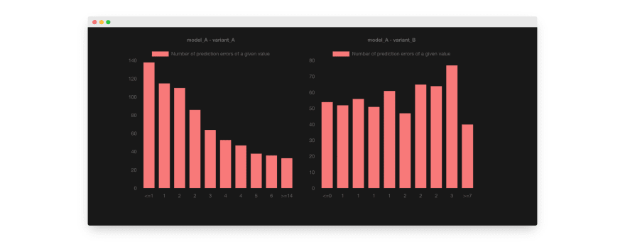
We will have a chart showing the difference between the actual value and the model’s prediction. Our chart will split the absolute errors into buckets (percentiles) and display the number of errors within every bucket.
If the new variant of the model performs better than the existing model, we should see fewer large errors in the charts. A perfect (and unrealistic) model would produce a single error bar in the left-most part of the chart with the “0” label.
At the beginning of the article, we looked at an example chart that shows no significant difference between both model variants:

If the variant B were better than the variant A, its chart could look like this (note the axis values in both pictures):
Creating a Cube deployment
Cube Cloud is the easiest way to get started with Cube. It provides a fully managed, ready to use Cube cluster. However, if you prefer self-hosting, then follow this tutorial.
First, please create a new Cube Cloud deployment. Then, open the "Deployments" page and click the “Create deployment” button.

We choose the Presto cluster:

Finally, we fill out the connection parameters and click the “Apply” button. Remember to enable the SSL connection!

Defining the data model in Cube
We have our queries ready to copy-paste, and we have configured a Presto connection in Cube. Now, we can define the Cube schema to retrieve query results.
Let’s open the Schema view in Cube and add a new file.

In the next window, type the file name errorpercentiles.js and click “Create file.”

In the following paragraphs, we will explain parts of the configuration and show you code fragments to copy-paste. You don’t have to do that in such small steps!
Below, you see the entire content of the file. Later, we explain the configuration parameters.
const measureNames = [
  'perc_10', 'perc_10_value',
  'perc_20', 'perc_20_value',
  'perc_30', 'perc_30_value',
  'perc_40', 'perc_40_value',
  'perc_50', 'perc_50_value',
  'perc_60', 'perc_60_value',
  'perc_70', 'perc_70_value',
  'perc_80', 'perc_80_value',
  'perc_90', 'perc_90_value',
  'perc_100', 'perc_100_value',
];

const measures = Object.keys(measureNames).reduce((result, name) => {
  const sqlName = measureNames[name];
  return {
    ...result,
    [sqlName]: {
      sql: () => sqlName,
      type: `max`
    }
  };
}, {});

cube('errorpercentiles', {
  sql: `with sagemaker as (
    select
    model_name,
    variant_name,
    cast(json_extract(FROM_UTF8( from_base64(capturedata.endpointinput.data)), '$.correlation_id') as varchar) as correlation_id,
    cast(json_extract(FROM_UTF8( from_base64(capturedata.endpointoutput.data)), '$.prediction') as double) as prediction
    from s3.sagemaker_logs.logs
  )
, actual as (
  select correlation_id, actual_value
  from postgresql.public.actual_values
)
, logs as (
  select model_name, variant_name as model_variant, sagemaker.correlation_id, prediction, actual_value as actual
  from sagemaker
  left outer join actual
  on sagemaker.correlation_id = actual.correlation_id
)
, errors as (
  select abs(prediction - actual) as abs_err, model_name, model_variant from logs
),
percentiles as (
  select approx_percentile(abs_err, 0.1) as perc_10,
  approx_percentile(abs_err, 0.2) as perc_20,
  approx_percentile(abs_err, 0.3) as perc_30,
  approx_percentile(abs_err, 0.4) as perc_40,
  approx_percentile(abs_err, 0.5) as perc_50,
  approx_percentile(abs_err, 0.6) as perc_60,
  approx_percentile(abs_err, 0.7) as perc_70,
  approx_percentile(abs_err, 0.8) as perc_80,
  approx_percentile(abs_err, 0.9) as perc_90,
  approx_percentile(abs_err, 1.0) as perc_100,
  model_name,
  model_variant
  from errors
  group by model_name, model_variant
)
SELECT count(*) FILTER (WHERE e.abs_err <= perc_10) AS perc_10
, max(perc_10) as perc_10_value
, count(*) FILTER (WHERE e.abs_err > perc_10 and e.abs_err <= perc_20) AS perc_20
, max(perc_20) as perc_20_value
, count(*) FILTER (WHERE e.abs_err > perc_20 and e.abs_err <= perc_30) AS perc_30
, max(perc_30) as perc_30_value
, count(*) FILTER (WHERE e.abs_err > perc_30 and e.abs_err <= perc_40) AS perc_40
, max(perc_40) as perc_40_value
, count(*) FILTER (WHERE e.abs_err > perc_40 and e.abs_err <= perc_50) AS perc_50
, max(perc_50) as perc_50_value
, count(*) FILTER (WHERE e.abs_err > perc_50 and e.abs_err <= perc_60) AS perc_60
, max(perc_60) as perc_60_value
, count(*) FILTER (WHERE e.abs_err > perc_60 and e.abs_err <= perc_70) AS perc_70
, max(perc_70) as perc_70_value
, count(*) FILTER (WHERE e.abs_err > perc_70 and e.abs_err <= perc_80) AS perc_80
, max(perc_80) as perc_80_value
, count(*) FILTER (WHERE e.abs_err > perc_80 and e.abs_err <= perc_90) AS perc_90
, max(perc_90) as perc_90_value
, count(*) FILTER (WHERE e.abs_err > perc_90 and e.abs_err <= perc_100) AS perc_100
, max(perc_100) as perc_100_value
, p.model_name, p.model_variant
FROM percentiles p, errors e group by p.model_name, p.model_variant`,

preAggregations: {
// Pre-Aggregations definitions go here
// Learn more here: https://cube.dev/docs/caching/pre-aggregations/getting-started
},

joins: {
},

measures: measures,
dimensions: {
  modelVariant: {
    sql: `model_variant`,
    type: 'string'
  },
  modelName: {
    sql: `model_name`,
    type: 'string'
  },
}
});
In the sql property, we put the query prepared earlier. Note that your query MUST NOT contain a semicolon.

We will group and filter the values by the model and variant names, so we put those columns in the dimensions section of the cube configuration. The rest of the columns are going to be our measurements. We can write them out one by one like this:
measures: {
  perc_10: {
    sql: `perc_10`,
    type: `max`
  },
  perc_20: {
    sql: `perc_20`,
    type: `max`
  },
  perc_30: {
    sql: `perc_30`,
    type: `max`
  },
  perc_40: {
    sql: `perc_40`,
    type: `max`
  },
  perc_50: {
    sql: `perc_50`,
    type: `max`
  },
  perc_60: {
    sql: `perc_60`,
    type: `max`
  },
  perc_70: {
    sql: `perc_70`,
    type: `max`
  },
  perc_80: {
    sql: `perc_80`,
    type: `max`
  },
  perc_90: {
    sql: `perc_90`,
    type: `max`
  },
  perc_100: {
    sql: `perc_100`,
    type: `max`
  },
  perc_10_value: {
    sql: `perc_10_value`,
    type: `max`
  },
  perc_20_value: {
    sql: `perc_20_value`,
    type: `max`
  },
  perc_30_value: {
    sql: `perc_30_value`,
    type: `max`
  },
  perc_40_value: {
    sql: `perc_40_value`,
    type: `max`
  },
  perc_50_value: {
    sql: `perc_50_value`,
    type: `max`
  },
  perc_60_value: {
    sql: `perc_60_value`,
    type: `max`
  },
  perc_70_value: {
    sql: `perc_70_value`,
    type: `max`
  },
  perc_80_value: {
    sql: `perc_80_value`,
    type: `max`
  },
  perc_90_value: {
    sql: `perc_90_value`,
    type: `max`
  },
  perc_100_value: {
    sql: `perc_100_value`,
    type: `max`
  }
},
dimensions: {
  modelVariant: {
    sql: `model_variant`,
    type: 'string'
  },
  modelName: {
    sql: `model_name`,
    type: 'string'
  },
}

The notation we have shown you has lots of repetition and is quite verbose. We can shorten the measurements defined in the code by using JavaScript to generate them.
We had to add the following code before using the cube function!
First, we have to create an array of column names:
const measureNames = [
  'perc_10', 'perc_10_value',
  'perc_20', 'perc_20_value',
  'perc_30', 'perc_30_value',
  'perc_40', 'perc_40_value',
  'perc_50', 'perc_50_value',
  'perc_60', 'perc_60_value',
  'perc_70', 'perc_70_value',
  'perc_80', 'perc_80_value',
  'perc_90', 'perc_90_value',
  'perc_100', 'perc_100_value',
];
Now, we must generate the measures configuration object. We iterate over the array and create a measure configuration for every column:
const measures = Object.keys(measureNames).reduce((result, name) => {
  const sqlName = measureNames[name];
  return {
    ...result,
    [sqlName]: {
      sql: () => sqlName,
      type: `max`
    }
  };
}, {});
Finally, we can replace the measure definitions with:
measures: measures,
After changing the file content, click the “Save All” button.

And click the Continue button in the popup window.

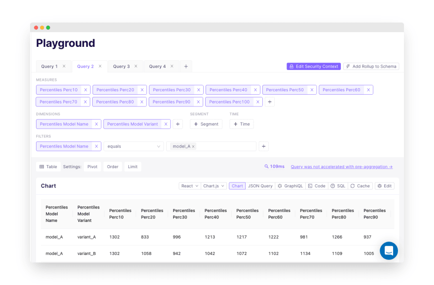
In the Playground view, we can test our query by retrieving the chart data as a table (or one of the built-in charts):
Configuring access control in Cube
In the Schema view, open the cube.js file.
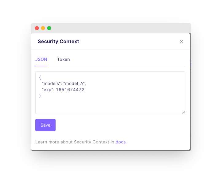
We will use the queryRewrite configuration option to allow or disallow access to data.
First, we will reject all API calls without the models field in the securityContext. We will put the identifier of the models the user is allowed to see in their JWT token. The security context contains all of the JWT token variables.
For example, we can send a JWT token with the following payload. Of course, in the application sending queries to Cube, we must check the user’s access right and set the appropriate token payload. Authentication and authorization are beyond the scope of this tutorial, but please don’t forget about them.
After rejecting unauthorized access, we add a filter to all queries.
We can distinguish between the datasets accessed by the user by looking at the data specified in the query. We need to do it because we must filter by the modelName property of the correct table.
In our queryRewrite configuration in the cube.js file, we use the query.filter.push function to add a modelName IN (model_1, model_2, …) clause to the SQL query:
module.exports = {
  queryRewrite: (query, { securityContext }) => {
    if (!securityContext.models) {
      throw new Error('No models found in Security Context!');
    }
    query.filters.push({
      member: 'percentiles.modelName',
      operator: 'in',
      values: securityContext.models,
    });
    return query;
  },
};
Configuring caching in Cube
By default, Cube caches all Presto queries for 2 minutes. Even though Sagemaker Endpoints stores logs in S3 in near real-time, we aren’t interested in refreshing the data so often. Sagemaker Endpoints store the logs in JSON files, so retrieving the metrics requires a full scan of all files in the S3 bucket.
When we gather logs over a long time, the query may take some time. Below, we will show you how to configure the caching in Cube. We recommend doing it when the end-user application needs over one second to load the data.
For the sake of the example, we will retrieve the value only twice a day.
Preparing data sources for caching
First, we must allow Presto to store data in both PostgreSQL and S3. It’s required because, in the case of Presto, Cube supports only the simple pre-aggregation strategy. Therefore, we need to pre-aggregate the data in the source databases before loading them into Cube.
In PostgreSQL, we grant permissions to the user account used by Presto to access the database:
GRANT CREATE ON SCHEMA the_schema_we_use TO the_user_used_in_presto;
GRANT USAGE ON SCHEMA the_schema_we_use TO the_user_used_in_presto;
If we haven’t modified anything in the AWS Glue data catalog, Presto already has permission to create new tables and store their data in S3, but the schema doesn’t contain the target S3 location yet, so all requests will fail.
We must login to AWS Console, open the Glue data catalog, and create a new database called prod_pre_aggregations. In the database configuration, we must specify the S3 location for the table content.
If you want to use a different database name, follow the instructions in our documentation.

Caching configuration in Cube
Let’s open the errorpercentiles.js schema file. Below the SQL query, we put the preAggregations configuration:
preAggregations: {
  cacheResults: {
    type: `rollup`,
    measures: [
      errorpercentiles.perc_10, errorpercentiles.perc_10_value,
      errorpercentiles.perc_20, errorpercentiles.perc_20_value,
      errorpercentiles.perc_30, errorpercentiles.perc_30_value,
      errorpercentiles.perc_40, errorpercentiles.perc_40_value,
      errorpercentiles.perc_50, errorpercentiles.perc_50_value,
      errorpercentiles.perc_60, errorpercentiles.perc_60_value,
      errorpercentiles.perc_70, errorpercentiles.perc_70_value,
      errorpercentiles.perc_80, errorpercentiles.perc_80_value,
      errorpercentiles.perc_90, errorpercentiles.perc_90_value,
      errorpercentiles.perc_100, errorpercentiles.perc_100_value
    ],
    dimensions: [errorpercentiles.modelName, errorpercentiles.modelVariant],
    refreshKey: {
      every: `12 hour`,
    },
  },
},
After testing the development version, we can also deploy the changes to production using the “Commit & Push” button. When we click it, we will be asked to type the commit message:

When we commit the changes, the deployment of a new version of the endpoint will start. A few minutes later, we can start sending queries to the endpoint.
We can also check the pre-aggregations window to verify whether Cube successfully created the cached data.

Now, we can move to the Playground tab and run our query. We should see the “Query was accelerated with pre-aggregation” message if Cube used the cached values to handle the request.

Building the front-end application
Cube can connect to a variety of tools, including Jupyter Notebooks, Superset, and Hex. However, we want a fully customizable dashboard, so we will build a front-end application.
Our dashboard consists of two parts: the website and the back-end service. In the web part, we will have only the code required to display the charts. In the back-end, we will handle authentication and authorization. The backend service will also send requests to the Cube REST API.
Getting the Cube API key and the API URL
Before we start, we have to copy the Cube API secret. Open the settings page in Cube Cloud's web UI and click the “Env vars” tab. In the tab, you will see all of the Cube configuration variables. Click the eye icon next to the CUBEJS_API_SECRET and copy the value.

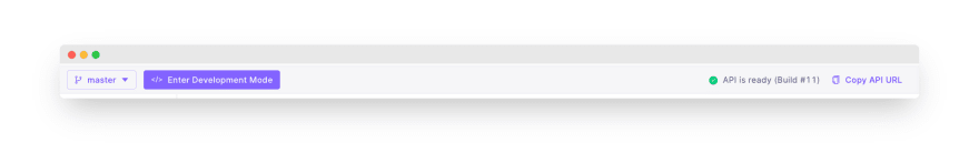
We also need the URL of the Cube endpoint. To get this value, click the “Copy API URL” link in the top right corner of the screen.
Back end for front end
Now, we can write the back-end code.
First, we have to authenticate the user. We assume that you have an authentication service that verifies whether the user has access to your dashboard and which models they can access. In our examples, we expect those model names in an array stored in the allowedModels variable.
After getting the user’s credentials, we have to generate a JWT to authenticate Cube requests. Note that we have also defined a variable for storing the CUBE_URL. Put the URL retrieved in the previous step as its value.
const jwt = require('jsonwebtoken');
CUBE_URL = '';
function create_cube_token() {
const CUBE_API_SECRET = your_token; // Don’t store it in the code!!!
// Pass it as an environment variable at runtime or use the
// secret management feature of your container orchestration system
const cubejsToken = jwt.sign(
{ "models": allowedModels },
CUBE_API_SECRET,
{ expiresIn: '30d' }
);
return cubejsToken;
}
We will need two endpoints in our back-end service: the endpoint returning the chart data and the endpoint retrieving the names of models and variants we can access.
We create a new express application running in the node server and configure the /models endpoint:
const request = require('request');
const express = require('express')
const bodyParser = require('body-parser')
const port = 5000;
const app = express()

app.use(bodyParser.json())
app.get('/models', getAvailableModels);

app.listen(port, () => {
  console.log(`Server is running on port ${port}`)
})
In the getAvailableModels function, we query the Cube Cloud API to get the model names and variants. It will return only the models we are allowed to see because we have configured the Cube security context:
Our function returns a list of objects containing the modelName and modelVariant fields.
function getAvailableModels(req, res) {
  res.setHeader('Content-Type', 'application/json');
  request.post(CUBE_URL + '/load', {
    headers: {
      'Authorization': create_cube_token(),
      'Content-Type': 'application/json'
    },
    body: JSON.stringify({"query": {
      "dimensions": [
        "errorpercentiles.modelName",
        "errorpercentiles.modelVariant"
      ],
      "timeDimensions": [],
      "order": {
        "errorpercentiles.modelName": "asc"
      }
    }})
  }, (err, res_, body) => {
    if (err) {
      console.log(err);
    }
    body = JSON.parse(body);
    response = body.data.map(item => {
      return {
        modelName: item["errorpercentiles.modelName"],
        modelVariant: item["errorpercentiles.modelVariant"]
      }
    });
    res.send(JSON.stringify(response));
  });
};
Let’s retrieve the percentiles and percentile buckets. To simplify the example, we will show only the query and the response parsing code. The rest of the code stays the same as in the previous endpoint.
The query specifies all measures we want to retrieve and sets the filter to get data belonging to a single model’s variant. We could retrieve all data at once, but we do it one by one for every variant.
{
  "query": {
    "measures": [
      "errorpercentiles.perc_10",
      "errorpercentiles.perc_20",
      "errorpercentiles.perc_30",
      "errorpercentiles.perc_40",
      "errorpercentiles.perc_50",
      "errorpercentiles.perc_60",
      "errorpercentiles.perc_70",
      "errorpercentiles.perc_80",
      "errorpercentiles.perc_90",
      "errorpercentiles.perc_100",
      "errorpercentiles.perc_10_value",
      "errorpercentiles.perc_20_value",
      "errorpercentiles.perc_30_value",
      "errorpercentiles.perc_40_value",
      "errorpercentiles.perc_50_value",
      "errorpercentiles.perc_60_value",
      "errorpercentiles.perc_70_value",
      "errorpercentiles.perc_80_value",
      "errorpercentiles.perc_90_value",
      "errorpercentiles.perc_100_value"
    ],
    "dimensions": [
        "errorpercentiles.modelName",
        "errorpercentiles.modelVariant"
    ],
    "filters": [
      {
        "member": "errorpercentiles.modelName",
        "operator": "equals",
        "values": [
          req.query.model
        ]
      },
      {
        "member": "errorpercentiles.modelVariant",
        "operator": "equals",
        "values": [
          req.query.variant
        ]
      }
    ]
  }
}
The response parsing code extracts the number of values in every bucket and prepares bucket labels:
response = body.data.map(item => {
  return {
    modelName: item["errorpercentiles.modelName"],
    modelVariant: item["errorpercentiles.modelVariant"],
    labels: [
      "<=" + item['percentiles.perc_10_value'],
      item['errorpercentiles.perc_20_value'],
      item['errorpercentiles.perc_30_value'],
      item['errorpercentiles.perc_40_value'],
      item['errorpercentiles.perc_50_value'],
      item['errorpercentiles.perc_60_value'],
      item['errorpercentiles.perc_70_value'],
      item['errorpercentiles.perc_80_value'],
      item['errorpercentiles.perc_90_value'],
      ">=" + item['errorpercentiles.perc_100_value']
    ],
    values: [
      item['errorpercentiles.perc_10'],
      item['errorpercentiles.perc_20'],
      item['errorpercentiles.perc_30'],
      item['errorpercentiles.perc_40'],
      item['errorpercentiles.perc_50'],
      item['errorpercentiles.perc_60'],
      item['errorpercentiles.perc_70'],
      item['errorpercentiles.perc_80'],
      item['errorpercentiles.perc_90'],
      item['errorpercentiles.perc_100']
    ]
  }
})
Dashboard website
In the last step, we build the dashboard website using Vue.js.
If you are interested in copy-pasting working code, we have prepared the entire example in a CodeSandbox. Below, we explain the building blocks of our application.
We define the main Vue component encapsulating the entire website content. In the script section, we will download the model and variant names. In the template, we iterate over the retrieved models and generate a chart for all of them.
We put the charts in the Suspense component to allow asynchronous loading.
To keep the example short, we will skip the CSS style part.
<script setup>
import OwnerName from './components/OwnerName.vue'
import ChartView from './components/ChartView.vue'
import axios from 'axios'
import { ref } from 'vue'
const models = ref([]);
axios.get(SERVER_URL + '/models').then(response => {
models.value = response.data
});
</script>
<template>
<header>
<div class="wrapper">
<OwnerName name="Test Inc." />
</div>
</header>
<main>
<div v-for="model in models" v-bind:key="model.modelName">
<Suspense>
<ChartView v-bind:title="model.modelName" v-bind:variant="model.modelVariant" type="percentiles"/>
</Suspense>
</div>
</main>
</template>
The OwnerName component displays our client’s name. We will skip its code as it’s irrelevant in our example.
In the ChartView component, we use the vue-chartjs library to display the charts. Our setup script contains the required imports and registers the Chart.js components:
import { Bar } from 'vue-chartjs'
import { Chart as ChartJS, Title, Tooltip, Legend, BarElement, CategoryScale, LinearScale } from 'chart.js'
import { ref } from 'vue'
import axios from 'axios'
ChartJS.register(Title, Tooltip, Legend, BarElement, CategoryScale, LinearScale);
We have bound the title, variant, and chart type to the ChartView instance. Therefore, our component definition must contain those properties:
const props = defineProps({
  title: String,
  variant: String,
  type: String
})
Next, we retrieve the chart data and labels from the back-end service. We will also prepare the variable containing the label text:
const response = await axios.get(SERVER_URL + '/' + props.type + '?model=' + props.title + '&variant=' + props.variant)
const data = response.data[0].values;
const labels = response.data[0].labels;
const label_text = "Number of prediction errors of a given value"
Finally, we prepare the chart configuration variables:
const chartData = ref({
  labels: labels,
  datasets: [
    {
      label: label_text,
      backgroundColor: '#f87979',
      data: data
    }
  ],
});

const chartOptions = {
  plugins: {
    title: {
      display: true,
      text: props.title + ' - ' + props.variant,
    },
  },
  legend: {
    display: false
  },
  tooltip: {
    enabled: false
  }
}
In the template section of the Vue component, we pass the configuration to the Bar instance:
<template>
  <Bar ref="chart" v-bind:chart-data="chartData" v-bind:chart-options="chartOptions" />
</template>
If we have done everything correctly, we should see a dashboard page with error distributions.
Wrapping up
Thanks for following this tutorial.
We encourage you to spend some time reading the Cube and Ahana documentation.
Please don't hesitate to like and bookmark this post, write a comment, give Cube a star on GitHub, join Cube's Slack community, and subscribe to the Ahana newsletter.


Latest comments (0)