Hi guys! Welcome back to part 7 of this series of where we build our own deep learning library.
Last article went through the implementation of the automatic differentiation module. We will see how easy this module makes adding new layer types by implementing RNN layers in this part of the series.
The code for this series' library can be found at this repo:
 ashwins-code
/
Zen-Deep-Learning-Library
ashwins-code
/
Zen-Deep-Learning-Library
Deep Learning library written in Python. Contains code for my blog series on building a deep learning library.
Zen - Deep Learning Library
A deep learning library written in Python.
Contains the code for my blog series where we build this library from scratch
- mnist.py contains an example for a MNIST digit recogniser using the library
- rnn.py contains an example of a Recurrent Neural Network which learns to fit to the graph sin(x) * cos(x)
What are RNNs?
So far in our library, we have only encountered simple feed forward neural networks.
These networks work well in quite a few cases, but when our inputs introduce the concept of time, feed forward networks begin to struggle, since they contain no mechanism to encapsulate contextual data.
Several pieces of data, like language and stock price data just to name a few, are determined from historical data points. For example, in terms of generating language, the words in a sentence are determined by what words have already been generated. In terms of predicting stock prices, the previous prices can be used to determine whether the stock price rises/falls. Our feed forward networks simply do not have the mechanisms to handle such types of data, so how can we model such data?
RNNs were designed for this specific problem.
RNN stands for recurrent neural network.
As the name suggests, RNNs rely on a recurrence mechanism to capture contextual data.
How do they work?
RNNs utilise a hidden state to encapsulate sequential data.
What the hidden state exactly is will be explained a bit later.
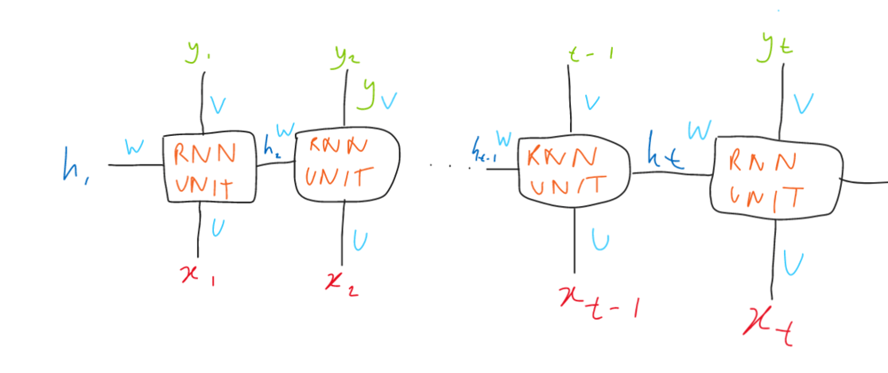
RNNs take in a sequence as input. They can output both a new sequence and the final hidden state from the input.
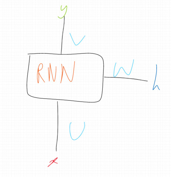
x is the input sequence
y is the outputted sequence
h is the final hidden state
U, W, V are all linear functions
How does this exactly happen?
I like to think of RNNs as a unit that is applied to each time-step of the input sequence. A time-step refers to the item in a sequence at a specific point in time.

refers to the item of the input sequence at time-step
refers to the item of the output sequence at time-step
refers to the hidden state after iterating through time-steps
As the diagram shows, RNN units produce an output sequence time-step and a hidden state after being fed the input sequence time-step and the previous hidden state, using the linear functions , , .
, , take the form
where is some adjustable weight matrix and and are vectors. is an adjustable vector.
The hidden state is a vector that encapsulates the meaning of the sequence. It essentially carries the information of all the time-steps it has seen so far.
and are caculated as follows.
The initial hidden state is usually a vector of 0s.
Hopefully you can see that if these calculations are applied to each time-step of the input sequence, an output sequence and a final hidden state is produced.
This final hidden state is a vector that contains all the information about the sequence the RNN layer was given.
The output sequence could be given to another RNN layer to reveal more complex patterns within the data.
During training, the weights and biases used within the , and functions are adjusted, so that the output sequence and hidden state better represent the inputted sequence.
Code Implementation
We shall add our RNN layer class to "nn.py"
import autodiff as ad
import numpy as np
import loss
import optim

...

class RNN(Layer):
    def __init__(self, units, hidden_dim, return_sequences=False):
        self.units = units
        self.hidden_dim = hidden_dim
        self.return_sequences = return_sequences
        self.U = None
        self.W = None
        self.V = None

    def one_forward(self, x):
        x = np.expand_dims(x, axis=1)
        state = np.zeros((x.shape[-1], self.hidden_dim))
        y = []

        for time_step in x:
            mul_u = self.U(time_step[0])
            mul_w = self.W(state)
            state = Tanh()(mul_u + mul_w)

            if self.return_sequences:
                y.append(self.V(state))

        if not self.return_sequences:
            state.value = state.value.squeeze()
            return state

        return y

    def __call__(self, x):
        if self.U is None:
            self.U = Linear(self.hidden_dim)
            self.W = Linear(self.hidden_dim)
            self.V = Linear(self.units)

        if not self.return_sequences:
            states = []
            for seq in x:
                state = self.one_forward(seq)
                states.append(state)

            s = ad.stack(states)
            return s

        sequences = []
        for seq in x:
            out_seq = self.one_forward(seq)
            sequences.append(out_seq)

        return sequences

    def update(self, optim):
        self.U.update(optim)
        self.W.update(optim)

        if self.return_sequences:
            self.V.update(optim)
Let's break this down into its separate methods.
def __init__(self, units, hidden_dim, return_sequences=False):
        self.units = units
        self.hidden_dim = hidden_dim
        self.return_sequences = return_sequences
        self.U = None
        self.W = None
        self.V = None
The class constructor takes in three parameters.
units - the size of each time-step in the outputted sequence when return_sequences is true
hidden_dim - the size of the hidden state
return_sequences - if true, the RNN layer will return a newly calculated sequence the same length as the input sequence. If false, it returns the final hidden stae.
self.U = None
self.W = None
self.V = None
U, W, V are initialised as None, but will represent the different weight matrices shown earlier after the layer's first forward pass.
The following methods have been commented to be better understood.
def __call__(self, x):
        """
        This method takes in a batch of sequences and returns the final hidden states after iterating through each sequence if return_sequences is False, otherwise it returns the output sequences.
        """

        if self.U is None:
            #intialise U, W, V if this is first forward pass
            #Since we know U, W, V are all linear functions with trainable parameters, we can simply assign them to instances of our already existing Linear class.
            self.U = Linear(self.hidden_dim)
            self.W = Linear(self.hidden_dim)
            self.V = Linear(self.units)

        if not self.return_sequences:
            states = []
            #go through each sequence
            for seq in x:
                #apply the "one_forward" method to sequence
                state = self.one_forward(seq)

                #append the final hidden state
                states.append(state)

            #use "stack" method to convert these list of tensors into a single tensor, so that its derivative can be calculated
            s = ad.stack(states)

            #return hidden states
            return s

        sequences = []
        #go through each sequence
        for seq in x:
            #apply the "one_forward" method to sequence
            out_seq = self.one_forward(seq)

            #append the output sequence
            sequences.append(out_seq)

        #return output sequences
        return sequences
def one_forward(self, x):
        """
        This method takes in a list representing a single sequence.
        """

        x = np.expand_dims(x, axis=1) #making list numpy array with 2 dimensions, so that its shape can be calculated for the following line
        state = np.zeros((x.shape[-1], self.hidden_dim)) #hidden state intitialised as a matrix of 0s
        y = [] #this array will store the output sequence if return_sequences is True


        #iterate through each time-step in the sequence
        for time_step in x:
            #perform next state calculation
            mul_u = self.U(time_step[0])
            mul_w = self.W(state)
            state = Tanh()(mul_u + mul_w)

            if self.return_sequences:
                #calculate the output sequence time-step if return_sequences is True
                y.append(self.V(state))

        if not self.return_sequences:
            # return hidden state if return_sequence is False
            state.value = state.value.squeeze()
            return state

        #return output sequence is return_sequences is True
        return y
def update(self, optim):
        self.U.update(optim)
        self.W.update(optim)

        if self.return_sequences:
            self.V.update(optim)
This update method was seen in the linear layer too. This method is called during backpropagation to adjust the weights of the layers.
You may have noticed a new function from our autodiff module - stack.
Here is the code for the stack function.
autodiff.py
def stack(tensor_list):
    tensor_values = [tensor.value for tensor in tensor_list]
    s = np.stack(tensor_values)

    var = Tensor(s)
    var.dependencies += tensor_list

    for tensor in tensor_list:
        var.grads.append(np.ones(tensor.value.shape))

    return var
This joins a list of tensors together into a single tensor.
This makes it possible for a group of separately computed tensors needed to be operated on at once, while still recording the operation onto the computation graph.
Notice how we did not need to write any backpropagation code for this class. Our autodiff module provides that layer of abstraction for us, making implementing new layer types much easier!
Building an RNN model to test it all out!
To see if this all is working well, we are going to build an RNN model to extrapolate trigonometric curves.
The RNN will take in a sequence of y-values from consecutive points from the curve. It's job is to predict the next y-value of the next point on the curve.
The RNN will extrapolate the curve by repeatedly feeding the most recent points on the curve
Imports...
import numpy as np
import nn
import optim
import loss
from matplotlib import pyplot as plt
Generate the first 200 points of a sin wave
x_axis = np.array(list(range(200))).T
seq = [np.sin(i) for i in range(200)]
Prepping dataset.
Inputs will contain a window of 49 points from the curve. The output is the y-value of the next point on the curve.
x = []
y = []

for i in range(len(seq) - 50):
    new_seq = [[i] for i in seq[i:i+50]]
    x.append(new_seq)
    y.append([seq[i+50]])
Building model
model = nn.Model([
    nn.RNN(32, hidden_dim=32, return_sequences=True),
    nn.RNN(0, hidden_dim=32), #units is 0 since it is irrelevant. return_sequence is False by default!
    nn.Linear(8),
    nn.Linear(1)
])
Train model and predict!
The predictions are plotted to a graph and saved as a png file.
model.train(np.array(x[:50]), np.array(y[:50]), epochs=10, optimizer=optim.RMSProp(0.0005), loss_fn=loss.MSE, batch_size=8)

preds = []

for i in x:
    preds.append(model(np.expand_dims(np.array(i), axis=0)).value[0][0])

plt.plot(x_axis[:150], seq[:150])
plt.plot(x_axis[:150], preds)
plt.savefig("graph.png")
Running the code will results in something similar to the following....
**

EPOCH 1
100%|███████████████████████████████████████████████████████████████████████████████████████████████████████████████████████████████████████████████████████████████████████████████| 7/7 [00:01<00:00,  6.24it/s]
LOSS 3.324489628181238

**

EPOCH 2
100%|███████████████████████████████████████████████████████████████████████████████████████████████████████████████████████████████████████████████████████████████████████████████| 7/7 [00:01<00:00,  6.49it/s]
LOSS 2.75052987566751

**

EPOCH 3
100%|███████████████████████████████████████████████████████████████████████████████████████████████████████████████████████████████████████████████████████████████████████████████| 7/7 [00:01<00:00,  6.28it/s]
LOSS 2.2723695780732083

**

...

EPOCH 9
100%|███████████████████████████████████████████████████████████████████████████████████████████████████████████████████████████████████████████████████████████████████████████████| 7/7 [00:01<00:00,  6.44it/s]
LOSS 0.07373163731751195

**

EPOCH 10
100%|███████████████████████████████████████████████████████████████████████████████████████████████████████████████████████████████████████████████████████████████████████████████| 7/7 [00:01<00:00,  6.63it/s]
LOSS 0.06355743981401539
Results
The results for a few expressions have been shown below.
Blue represents the true values
Orange represents the model's predictions
sin(x)
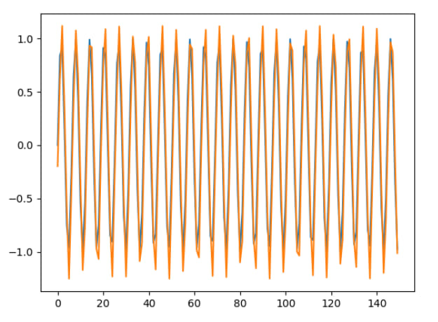
sin(x) * cos(x)

I am happy with these results!
Thanks for reading!
Thanks for reading through this blog post.
We will continue to add new layer types in the next few posts of this series, so be ready for those!


Top comments (0)