ashwins-code

Posted on Jan 8, 2022

Deep Learning Library From Scratch 3: More optimisers

#machinelearning #deeplearning #python #numpy

Welcome to part 3 of this series, where we build a deep learning library from scratch.

In this post, we will add more optimisation functions and loss functions to our library.

Here is the Github repo for this series

ashwins-code / Zen-Deep-Learning-Library

Deep Learning library written in Python. Contains code for my blog series on building a deep learning library.

Last post: https://dev.to/ashwinscode/deep-learning-library-from-scratch-2-backpropagation-116m

Optimisation functions

The goal of an optimisation function is to tweak the network parameters to minimise the neural network's loss.

It does this by taking the gradient of the parameters with respect to the loss and using this gradient to update the parameters.

Different loss functions use the gradients in different ways, which leads to an acceleration in the training process!

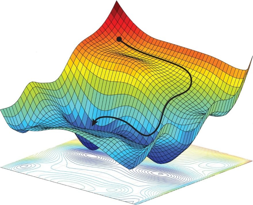
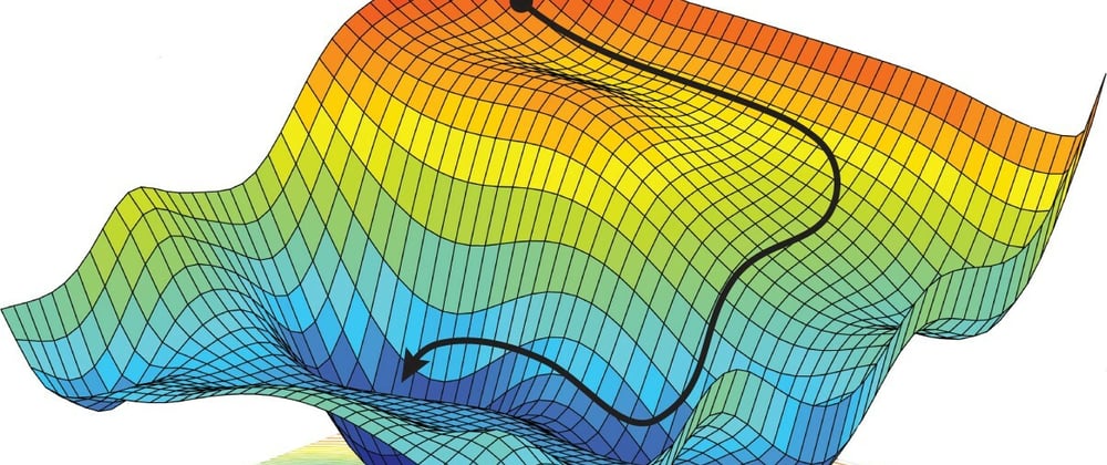
If we graph out the loss function, as seen in the image above, optimisers aim to change the parameters of the neural network, so that the minimum loss value is produced aka the lowest dip in the graph.

The path which the optimisers take during the training process is represented by the black ball.

Momentum

Momentum is an optimisation function, which extends the gradient descent algorithm (which we looked at in the last post).

It is designed to accelerate the training process, meaning it would minimise the loss in a fewer number of epochs. If we think about our "black ball", momentum causes this black ball to accelerate quickly towards the minimum, like rolling a ball down from the top of a hill.

Momentum accumulates the gradients calculated in previous epochs, which helps it to determine the direction to go to, in order to minimise the loss.

The formula it uses to update parameters is as follows

d_{t} = \beta \cdot d_{t-1} + l \cdot g \newline p_{t+1} = p_{t} - d_{t} \newline

$p_{t}$ is the parameter value at epoch t
$d_{t}$ is the "direction" to go at epoch t, calculated from previous epochs' gradients. It is initialised at 0.
$l$ is the learning rate
$\beta$ is a predetermined value (usually chosen to be 0.9)
$g$ is the gradient of the parameter with respect to this loss

Here is our python implementation of this optimiser

#optim.py

#...
class Momentum:
    def __init__(self, lr = 0.01, beta=0.9):
        self.lr = lr
        self.beta = beta

    def momentum_average(self, prev, grad):
        return (self.beta * prev) + (self.lr * grad)

    def __call__(self, model, loss):
        grad = loss.backward()

        for layer in tqdm.tqdm(model.layers[::-1]):
            grad = layer.backward(grad)

            if isinstance(layer, layers.Layer):
                if not hasattr(layer, "momentum"):
                    layer.momentum = {
                        "w": 0,
                        "b": 0
                    }
                layer.momentum["w"] = self.momentum_average(layer.momentum["w"], layer.w_gradient)
                layer.momentum["b"] = self.momentum_average(layer.momentum["b"], layer.b_gradient)

                layer.w -= layer.momentum["w"]
                layer.b -= layer.momentum["b"]
#...

RMSProp

RMSProp works by taking an exponential average of the squares of the previous gradients. An exponential average is used to give recent gradients more weight than earlier gradients.

This exponential average is used to determine the update in the parameter.

RMSProp aims to minimise the oscillations in the training step. In terms of our "black ball", the "ball" would take a smooth, straight path towards the minimum, instead of zig-zagging towards it, which often happens with other optimisers.

Here are the equations for parameter updates...

d_{t} = \beta \cdot d_{t-1} + (1 - \beta) \cdot g^{2} \newline \varDelta p_{t} = \frac{l}{\sqrt{d_{t} + \epsilon}} \cdot g \newline p_{t+1} = p_{t} - \varDelta p_{t} \newline

$p_{t}$ is the parameter value at epoch t
$d_{t}$ is the exponential squared average of previous gradients. It is initialised at 0.
$l$ is the learning rate
$\beta$ is a predetermined value (usually chosen to be 0.9)
$g$ is the gradient of the parameter with respect to this loss
$\epsilon$ is a predetermined value, to avoid division by 0. Usually set at $10^{-10}$

As seen in the second equation, we divide the learning rate by the exponential average. This leads to parameters in later epochs having a larger training step, since the exponential average gets smaller as more epochs occur.

RMSProp also automatically slows down as it approaches the minima, which is ideal, since a too large step size would cause an overcorrection in the updating of parameters.

Here is our python implementation...

#optim.py

#...
class RMSProp:
    def __init__(self, lr = 0.01, beta=0.9, epsilon=10**-10):
        self.lr = lr
        self.beta = beta
        self.epsilon = epsilon

    def rms_average(self, prev, grad):
        return self.beta * prev + (1 - self.beta) * (grad ** 2)

    def __call__(self, model, loss):
        grad = loss.backward()

        for layer in tqdm.tqdm(model.layers[::-1]):
            grad = layer.backward(grad)

            if isinstance(layer, layers.Layer):
                if not hasattr(layer, "rms"):
                    layer.rms = {
                        "w": 0,
                        "b": 0
                    }

                layer.rms["w"] = self.rms_average(layer.rms["w"], layer.w_gradient)
                layer.rms["b"] = self.rms_average(layer.rms["b"], layer.b_gradient)

                layer.w -= self.lr / (np.sqrt(layer.rms["w"] + self.epsilon)) * layer.w_gradient
                layer.b -= self.lr / (np.sqrt(layer.rms["b"] + self.epsilon)) * layer.b_gradient
#...

Adam

Adam combines the ideas in RMSProp and Momentum together.

Here are the update equations...

v_{t} = \beta_{1} \cdot v_{t-1} + (1 - \beta_{1}) \cdot g \newline s_{t} = \beta_{2} \cdot s_{t-1} + (1 - \beta_{2}) \cdot g^{2} \newline \varDelta p_{t} = l \cdot \frac{v_{t}}{\sqrt{s_{t}} + \epsilon } \newline p_{t+1} = p_{t} - \varDelta p_{t}

$p_{t}$ is the parameter value at epoch t
$v_{t}$ is the exponential average of previous gradients. It is initialised at 0.
$s_{t}$ is the exponential squared average of previous gradients. It is initialised at 0.
$l$ is the learning rate
$\beta_{1}$ is a predetermined value (usually chosen to be 0.9)
$\beta_{2}$ is a predetermined value (usually chosen to be 0.999)
$g$ is the gradient of the parameter with respect to this loss
$\epsilon$ is a predetermined value, to avoid division by 0. Usually set at $10^{-10}$

Here is our python implementation...

#optim.py

#...
class Adam:
    def __init__(self, lr = 0.01, beta1=0.9, beta2=0.999, epsilon=10**-8):
        self.lr = lr
        self.beta1 = beta1
        self.beta2 = beta2
        self.epsilon = epsilon

    def rms_average(self, prev, grad):
        return (self.beta2 * prev) + (1 - self.beta2) * (grad ** 2)

    def momentum_average(self, prev, grad):
        return (self.beta1 * prev) + ((1 - self.beta1) * grad)

    def __call__(self, model, loss):
        grad = loss.backward()

        for layer in tqdm.tqdm(model.layers[::-1]):
            grad = layer.backward(grad)

            if isinstance(layer, layers.Layer):
                if not hasattr(layer, "adam"):
                    layer.adam = {
                        "w": 0,
                        "b": 0,
                        "w2": 0,
                        "b2": 0
                    }

                layer.adam["w"] = self.momentum_average(layer.adam["w"], layer.w_gradient)
                layer.adam["b"] = self.momentum_average(layer.adam["b"], layer.b_gradient)
                layer.adam["w2"] = self.rms_average(layer.adam["w2"], layer.w_gradient)
                layer.adam["b2"] = self.rms_average(layer.adam["b2"], layer.b_gradient)

                w_adjust = layer.adam["w"] / (1 - self.beta1)
                b_adjust = layer.adam["b"] / (1 - self.beta1)
                w2_adjust = layer.adam["w2"] / (1 - self.beta2)
                b2_adjust = layer.adam["b2"] / (1 - self.beta2)

                layer.w -= self.lr * (w_adjust / np.sqrt(w2_adjust) + self.epsilon)
                layer.b -= self.lr * (b_adjust /  np.sqrt(b2_adjust) + self.epsilon)
#...

Using our new optimisers!

This is how we'd use our new optimisers in our library, training a model for the same problem we described last post (XOR gate).

import layers
import loss
import optim
import numpy as np


x = np.array([[0, 1], [0, 0], [1, 1], [1, 0]])
y = np.array([[0, 1], [1, 0], [1, 0], [0, 1]]) 

net = layers.Model([
    layers.Linear(8),
    layers.Linear(4),
    layers.Sigmoid(),
    layers.Linear(2),
    layers.Softmax()
])

net.train(x, y, optim=optim.RMSProp(lr=0.02), loss=loss.MSE(), epochs=200)

print (net(x))

epoch 190 loss 0.00013359948998165245
100%|████████████████████████████████████████████████████████████████████████████████████████████| 5/5 [00:00<?, ?it/s]
epoch 191 loss 0.00012832321751534635
100%|████████████████████████████████████████████████████████████████████████████████████████████| 5/5 [00:00<?, ?it/s]
epoch 192 loss 0.0001232564322705172
100%|████████████████████████████████████████████████████████████████████████████████████████████| 5/5 [00:00<?, ?it/s]
epoch 193 loss 0.00011839076882215646
100%|██████████████████████████████████████████████████████████████████████████████████| 5/5 [00:00<00:00, 5018.31it/s]
epoch 194 loss 0.00011371819900553786
100%|████████████████████████████████████████████████████████████████████████████████████████████| 5/5 [00:00<?, ?it/s]
epoch 195 loss 0.00010923101808808603
100%|████████████████████████████████████████████████████████████████████████████████████████████| 5/5 [00:00<?, ?it/s]
epoch 196 loss 0.00010492183152425807
100%|████████████████████████████████████████████████████████████████████████████████████████████| 5/5 [00:00<?, ?it/s]
epoch 197 loss 0.00010078354226798005
100%|████████████████████████████████████████████████████████████████████████████████████████████| 5/5 [00:00<?, ?it/s]
epoch 198 loss 9.680933861835338e-05
100%|████████████████████████████████████████████████████████████████████████████████████████████| 5/5 [00:00<?, ?it/s]
epoch 199 loss 9.299268257548828e-05
100%|████████████████████████████████████████████████████████████████████████████████████████████| 5/5 [00:00<?, ?it/s]
epoch 200 loss 8.932729868441197e-05
[[0.00832775 0.99167225]
 [0.98903246 0.01096754]
 [0.99082742 0.00917258]
 [0.00833392 0.99166608]]

As you can see, compared to the last post, our model has trained much much better, thanks to our new optimiser!

Thanks for reading! Next post we will apply our library so far to a more advanced problem (handwritten digit recognition!)

DEV Community

Deep Learning Library From Scratch 3: More optimisers

ashwins-code / Zen-Deep-Learning-Library

Deep Learning library written in Python. Contains code for my blog series on building a deep learning library.

Optimisation functions

Momentum

RMSProp

Adam

Using our new optimisers!

Latest comments (0)

Read next

Building a Universally Portable Python App

Secure Your Data: AES-GCM Encryption & Decryption for JavaScript, TypeScript, Java, and Python 🛡️🔐

How to install python in a docker container.

What Asterisk (*) Can Do In Python