This will be a pretty small post, but an interesting one nevertheless.
Originally published at https://alexandruburlacu.github.io/posts/2021-06-18-kmeans-trick
K-Means is an elegant algorithm. It's easy to understand (make random points, move them iteratively to become centers of some existing clusters) and works well in practice. When I first learned about it, I recall being fascinated. It was elegant. But then, in time, the interest faded away, I was noticing numerous limitations, among which is the spherical cluster prior, its linear nature, and what I found especially annoying in EDA scenarios, the fact that it doesn’t find the optimal number of clusters by itself, so you need to tinker with this parameter too. And then, a couple of years ago, I found out about a few neat tricks on how to use K-Means. So here it goes.
The first trick
First, we need to establish a baseline. I'll use mostly the breast cancer dataset, but you can play around with any other dataset.
from sklearn.cluster import KMeans
from sklearn.svm import LinearSVC
from sklearn.datasets import load_breast_cancer
from sklearn.model_selection import train_test_split

import numpy as np

X, y = load_breast_cancer(return_X_y=True)

X_train, X_test, y_train, y_test = train_test_split(X, y, random_state=17)

svm = LinearSVC(random_state=17)
svm.fit(X_train, y_train)
svm.score(X_test, y_test) # should be ~0.93
So, what's this neat trick that reignited my interest for K-Means?
K-Means can be used as a source of new features.
How, you might ask? Well, K-Means is a clustering algorithm, right? You can add the inferred cluster as a new categorical feature.
Now, let's try this.
# imports from the example above

svm = LinearSVC(random_state=17)
kmeans = KMeans(n_clusters=3, random_state=17)
X_clusters = kmeans.fit_predict(X_train).reshape(-1, 1)

svm.fit(np.hstack([X_train, X_clusters]), y_train)
svm.score(np.hstack([X_test, kmeans.predict(X_test).reshape(-1, 1)]), y_test) # should be ~0.937

Source: knowyourmeme.com
These features are categorical, but we can ask the model to output distances to all the centroids, thus obtaining (hopefully) more informative features.
# imports from the example above

svm = LinearSVC(random_state=17)
kmeans = KMeans(n_clusters=3, random_state=17)
X_clusters = kmeans.fit_transform(X_train)
#                       ^^^^^^^^^
#                       Notice the `transform` instead of `predict`
# Scikit-learn supports this method as early as version 0.15

svm.fit(np.hstack([X_train, X_clusters]), y_train)
svm.score(np.hstack([X_test, kmeans.transform(X_test)]), y_test) # should be ~0.727
Wait, what's wrong? Could it be that there's a correlation between existing features and the distances to the centroids?
import matplotlib.pyplot as plt
import seaborn as sns
import pandas as pd

columns = ['mean radius', 'mean texture', 'mean perimeter', 'mean area',
       'mean smoothness', 'mean compactness', 'mean concavity',
       'mean concave points', 'mean symmetry', 'mean fractal dimension',
       'radius error', 'texture error', 'perimeter error', 'area error',
       'smoothness error', 'compactness error', 'concavity error',
       'concave points error', 'symmetry error',
       'fractal dimension error', 'worst radius', 'worst texture',
       'worst perimeter', 'worst area', 'worst smoothness',
       'worst compactness', 'worst concavity', 'worst concave points',
       'worst symmetry', 'worst fractal dimension',
       'distance to cluster 1', 'distance to cluster 2', 'distance to cluster 3']
data = pd.DataFrame.from_records(np.hstack([X_train, X_clusters]), columns=columns)
sns.heatmap(data.corr())
plt.xticks(rotation=-45)
plt.show()

Notice the last 3 columns, especially the last one, and their color on every row.
You probably heard that we want the features in the dataset to be as independent as possible. The reason is that a lot of machine learning models assume this independence to have a simpler algorithm. Some more info on this topic can be found here and here, but the gist of it is that having redundant information in linear models destabilizes the model, and in turn, it is more likely to mess up. On numerous occasions, I noticed this problem, sometimes even with non-linear models, and purging the dataset from correlated features usually gives a slight increase in the model's performance characteristic.
Back to our main topic. Given that our new features are indeed correlated with some of the existing ones, what if we use only the distances to the cluster means as features, will it work then?
# imports from the example above

svm = LinearSVC(random_state=17)
kmeans = KMeans(n_clusters=3, random_state=17)
X_clusters = kmeans.fit_transform(X_train)

svm.fit(X_clusters, y_train)
svm.score(kmeans.transform(X_test), y_test) # should be ~0.951
Much better. With this example, you can see that we can use KMeans as a way to do dimensionality reduction. Neat.
So far so good. But the piece de resistance is yet to be shown.
The second trick
K-Means can be used as a substitute for the kernel trick
You heard me right. You can, for example, define more centroids for the K-Means algorithm to fit than there are features, much more.
# imports from the example above

svm = LinearSVC(random_state=17)
kmeans = KMeans(n_clusters=250, random_state=17)
X_clusters = kmeans.fit_transform(X_train)

svm.fit(X_clusters, y_train)
svm.score(kmeans.transform(X_test), y_test) # should be ~0.944
Well, not as good, but pretty decent. In practice, the greatest benefit of this approach is when you have a lot of data. Also, predictive performance-wise your mileage may vary, I, for one, had run this method with n_clusters=1000 and it worked better than only with a few clusters.
SVMs are known to be slow to train on big datasets. Impossibly slow. Been there, done that. That's why, for example, there are numerous techniques to approximate the kernel trick with much less computational resources.
By the way, let's compare how this K-Means trick will do against classic SVM and some alternative kernel approximation methods.
The code below is inspired by these two scikit-learn examples.
import matplotlib.pyplot as plt
import numpy as np
from time import time

from sklearn.datasets import load_breast_cancer
from sklearn.svm import LinearSVC, SVC
from sklearn import pipeline
from sklearn.kernel_approximation import RBFSampler, Nystroem, PolynomialCountSketch
from sklearn.preprocessing import MinMaxScaler, Normalizer
from sklearn.model_selection import train_test_split
from sklearn.cluster import MiniBatchKMeans


mm = pipeline.make_pipeline(MinMaxScaler(), Normalizer())

X, y = load_breast_cancer(return_X_y=True)
X = mm.fit_transform(X)

data_train, data_test, targets_train, targets_test = train_test_split(X, y, random_state=17)
We will test 3 methods for kernel approximation available in the scikit-learn package, against the K-Means trick, and as baselines, we will have a linear SVM and an SVM that uses the kernel trick.
# Create a classifier: a support vector classifier
kernel_svm = SVC(gamma=.2, random_state=17)
linear_svm = LinearSVC(random_state=17)

# create pipeline from kernel approximation and linear svm
feature_map_fourier = RBFSampler(gamma=.2, random_state=17)
feature_map_nystroem = Nystroem(gamma=.2, random_state=17)
feature_map_poly_cm = PolynomialCountSketch(degree=4, random_state=17)
feature_map_kmeans = MiniBatchKMeans(random_state=17)
fourier_approx_svm = pipeline.Pipeline([("feature_map", feature_map_fourier),
                                        ("svm", LinearSVC(random_state=17))])

nystroem_approx_svm = pipeline.Pipeline([("feature_map", feature_map_nystroem),
                                        ("svm", LinearSVC(random_state=17))])

poly_cm_approx_svm = pipeline.Pipeline([("feature_map", feature_map_poly_cm),
                                        ("svm", LinearSVC(random_state=17))])

kmeans_approx_svm = pipeline.Pipeline([("feature_map", feature_map_kmeans),
                                        ("svm", LinearSVC(random_state=17))])
Let's collect the timing and score results for each of our configurations.
# fit and predict using linear and kernel svm:
kernel_svm_time = time()
kernel_svm.fit(data_train, targets_train)
kernel_svm_score = kernel_svm.score(data_test, targets_test)
kernel_svm_time = time() - kernel_svm_time

linear_svm_time = time()
linear_svm.fit(data_train, targets_train)
linear_svm_score = linear_svm.score(data_test, targets_test)
linear_svm_time = time() - linear_svm_time

sample_sizes = 30 * np.arange(1, 10)
fourier_scores = []
nystroem_scores = []
poly_cm_scores = []
kmeans_scores = []

fourier_times = []
nystroem_times = []
poly_cm_times = []
kmeans_times = []

for D in sample_sizes:
    fourier_approx_svm.set_params(feature_map__n_components=D)
    nystroem_approx_svm.set_params(feature_map__n_components=D)
    poly_cm_approx_svm.set_params(feature_map__n_components=D)
    kmeans_approx_svm.set_params(feature_map__n_clusters=D)
    start = time()
    nystroem_approx_svm.fit(data_train, targets_train)
    nystroem_times.append(time() - start)

    start = time()
    fourier_approx_svm.fit(data_train, targets_train)
    fourier_times.append(time() - start)

    start = time()
    poly_cm_approx_svm.fit(data_train, targets_train)
    poly_cm_times.append(time() - start)

    start = time()
    kmeans_approx_svm.fit(data_train, targets_train)
    kmeans_times.append(time() - start)

    fourier_score = fourier_approx_svm.score(data_test, targets_test)
    fourier_scores.append(fourier_score)
    nystroem_score = nystroem_approx_svm.score(data_test, targets_test)
    nystroem_scores.append(nystroem_score)
    poly_cm_score = poly_cm_approx_svm.score(data_test, targets_test)
    poly_cm_scores.append(poly_cm_score)
    kmeans_score = kmeans_approx_svm.score(data_test, targets_test)
    kmeans_scores.append(kmeans_score)
Now let's plot all the collected results.
plt.figure(figsize=(16, 4))
accuracy = plt.subplot(211)
timescale = plt.subplot(212)

accuracy.plot(sample_sizes, nystroem_scores, label="Nystroem approx. kernel")
timescale.plot(sample_sizes, nystroem_times, '--',
               label='Nystroem approx. kernel')

accuracy.plot(sample_sizes, fourier_scores, label="Fourier approx. kernel")
timescale.plot(sample_sizes, fourier_times, '--',
               label='Fourier approx. kernel')

accuracy.plot(sample_sizes, poly_cm_scores, label="Polynomial Count-Min approx. kernel")
timescale.plot(sample_sizes, poly_cm_times, '--',
               label='Polynomial Count-Min approx. kernel')

accuracy.plot(sample_sizes, kmeans_scores, label="K-Means approx. kernel")
timescale.plot(sample_sizes, kmeans_times, '--',
               label='K-Means approx. kernel')

# horizontal lines for exact rbf and linear kernels:
accuracy.plot([sample_sizes[0], sample_sizes[-1]],
              [linear_svm_score, linear_svm_score], label="linear svm")
timescale.plot([sample_sizes[0], sample_sizes[-1]],
               [linear_svm_time, linear_svm_time], '--', label='linear svm')

accuracy.plot([sample_sizes[0], sample_sizes[-1]],
              [kernel_svm_score, kernel_svm_score], label="rbf svm")
timescale.plot([sample_sizes[0], sample_sizes[-1]],
               [kernel_svm_time, kernel_svm_time], '--', label='rbf svm')
And some more plot adjustments, to make it pretty.
# legends and labels
accuracy.set_title("Classification accuracy")
timescale.set_title("Training times")
accuracy.set_xlim(sample_sizes[0], sample_sizes[-1])
accuracy.set_xticks(())
accuracy.set_ylim(np.min(fourier_scores), 1)
timescale.set_xlabel("Sampling steps = transformed feature dimension")
accuracy.set_ylabel("Classification accuracy")
timescale.set_ylabel("Training time in seconds")
accuracy.legend(loc='best')
timescale.legend(loc='best')
plt.tight_layout()
plt.show()
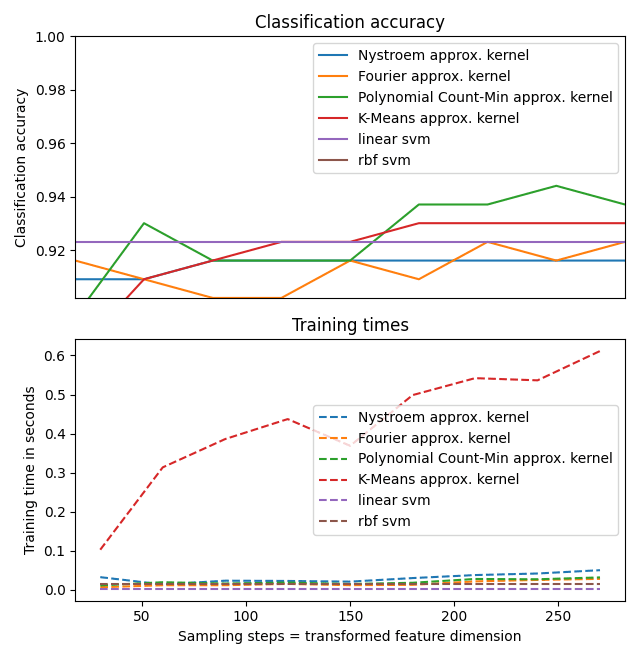
Meh. So was it all for nothing?
You know what? Not in the slightest. Even if it's the slowest, K-Means as an approximation of the RBF Kernel is still a good option. I'm not kidding. You can use this special kind of K-Means in scikit-learn called MiniBatchKMeans which is one of the few algorithms that support the .partial_fit method. Combining this with a machine learning model that has .partial_fit too, like a PassiveAggressiveClassifier one can create a pretty interesting solution.
Note that the beauty of .partial_fit is twofold. First, it makes it possible to train algorithms in an out-of-core fashion, which is to say, with more data than fits in the RAM. Second, depending on your type of problem, if you could in principle (very-very in principle) never need to switch the model, it could be additionally trained right where it is deployed. That's called online learning, and it's super interesting. Something like this is what some Chinese companies are doing and in general can be pretty useful for AdTech, because you can receive the info whenever your ad recommendation was right or wrong within seconds.
You know what, here's a little example of this approach for out-of-core learning.
from sklearn.cluster import MiniBatchKMeans
from sklearn.linear_model import PassiveAggressiveClassifier

from sklearn.model_selection import train_test_split
from sklearn.datasets import load_breast_cancer

import numpy as np

def batch(iterable, n=1):
    # source: https://stackoverflow.com/a/8290508/5428334
    l = len(iterable)
    for ndx in range(0, l, n):
        yield iterable[ndx:min(ndx + n, l)]

X, y = load_breast_cancer(return_X_y=True)

X_train, X_test, y_train, y_test = train_test_split(X, y, random_state=17)

kmeans = MiniBatchKMeans(n_clusters=100, random_state=17) # K-Means has a constraint, n_clusters <= n_samples to fit
pac = PassiveAggressiveClassifier(random_state=17)

for x, y in zip(batch(X_train, n=100), batch(y_train, n=100)):
    kmeans.partial_fit(x, y)       # fit K-Means a bit
    x_dist = kmeans.transform(x)   # obtain distances
    pac.partial_fit(x_dist, y, classes=[0, 1])     # learn a bit the classifier, we need to indicate the classes
    print(pac.score(kmeans.transform(X_test), y_test))

# 0.909 after 100 samples
# 0.951 after 200 samples
# 0.951 after 300 samples
# 0.944 after 400 samples
# 0.902 after 426 samples


# VS
kmeans = MiniBatchKMeans(n_clusters=100, random_state=17)
pac = PassiveAggressiveClassifier(random_state=17)

pac.fit(kmeans.fit_transform(X_train), y_train)
pac.score(kmeans.transform(X_test), y_test)
# should be ~0.951
Epilogue
So you've made it till the end. Hope now your ML toolset is richer. Maybe you've heard about the so-called "no free lunch" theorem; basically, there's no silver bullet, in this case for ML problems. Maybe for the next project, the methods outlined in this post won't work, but for the one that will come after that, they will. So just experiment, and see for yourself. And if you need an online learning algorithm/method, well, there's a bigger chance that K-Means as a kernel approximation is the right tool for you.
By the way, there's another blog post, also on ML, in the works now. What's even nicer, among many other nice things in it, it describes a rather interesting way to use K-Means. But no spoilers for now. Stay tuned.
Finally, if you’re reading this, thank you! If you want to leave some feedback or just have a question, you've got quite a menu of options (see the footer of this page for contacts + you have the Disqus comment section).
Some links you might find interesting
- A stackexchange discussion about using K-Means as a feature engineering tool
- A more in-depth explanation of K-Means
- A research paper that uses K-Means for an efficient SVM
Acknowledgements
Special thanks to @dgaponcic for style checks and content review, and thank you @anisoara_ionela for grammar checking this article more thoroughly than any AI ever could. You're the best <3
P.S. I believe you noticed all these random_states in the code. If you're wondering why I added these, it's to make the code samples reproducible. Because frequently tutorials don't do this and it leaves space for cherry-picking, where the author presents only the best results, and when trying to replicate these, the reader either can't or it takes a lot of time. But know this, you can play around with the values of random_state and get widely different results. For example, when running the snippet with original features and distances to the 3 centroids, the one with a 0.727 score, with a random seed of 41 instead of 17, you can get the accuracy score of 0.944. So yeah, random_state or however else the random seed is called in your framework of choice is an important aspect to keep in mind, especially when doing research.


Oldest comments (0)