Graphs are non-linear data structures in which a problem is represented as a network by connecting nodes and edges, examples of this can be networks of communication, flows of computation, paths in a road, connections in social networks, etc. The next image shows graph connections of Facebook for the year 2010:

This image shows interesting information such as, which countries the app has more or less influence, you can also see cultural relations between countries: Hawaii to the continental US; Australia to New Zealand; Colombia to Spain, you could also observe country outlines like India isolated in the dark void of China and Russia[1].
In short, Graph algorithms offer the tools required to understand, model, and establish connection behaviors of systems at a high level of complexity.
This article will discuss the theory behind the most popular algorithms to find strongly connected components (SCC), the time complexity of each and finally compare both algorithms using benchmarks on directed graphs. Let's start defining what directed graphs are:
Directed Graphs
A directed graph (also known as Digraph) is a type of graph in which the edges have a defined direction (Figure 2), unlike an undirected graph, in which the edges are symmetrical relations and do not point in any direction, the edges are bidirectional (Figure 3).


A graph is connected if there is a path between every pair of vertices, in digraphs there are two classifications depending on the nature of the connections, weakly connected and strongly connected. A digraph is called weakly connected, if it is possible to reach any node starting from any other node by traversing edges in some direction not necessarily in the direction they point [3].

On the other hand, a digraph is called strong connected, if for each pair of vertices u and v, there is a path from u to v and a path from v to u, in other words, if there is a path in each direction between each pair of vertices of the graph.

To find this strong connected components, DFS (Depth first search) can be used, the two most famous algorithms that use this traversal technique are:
- Kosaraju-Sharir algorithm
- Tarjan’s algorithm
Kosaraju-Sharir algorithm
In the year 1978, computer scientist S.Rao Kosaraju proposed an implementation of the algorithm but did not publish it. Independently, computer scientist Micha Sharir discovered it and published it in 1981. The main idea of the algorithm is based on the fact that the strongly connected components of a graph A are exactly the same as those of the transposed graph of A (reversing all the edges of graph A).
Algorithm steps:
1. Create a graph
For the creation of the graph an adjacency list will be used, an adjacency list consists in a collection of unordered lists (child nodes) grouped by a map, where each key represents the parent node. The code shown below handles an implementation of the graph with a struct having the following fields:
- nodes: this field has the purpose of keeping track of all labels associated to vertices in the graph.
- reversed: As said before, Kosaraju-Sharir algorithm makes use of the transposed graph, to save unnecessary iterations like traversing the graph to find the transposed, simply when adding a new edge to the base graph, also add the same edges in reversed direction (See section 2, line 10).
- edges: Adjacency list of the graph.
package kosarajuSharir

import (
    g "SCC_analysis/graph"
    "fmt"
    "github.com/abaron10/Gothon/gothonSlice"
)

type graph struct {
    nodes    []int
    reversed *graph
    edges    map[int][]*edge
}

type edge struct {
    from int
    to   int
}

func newEdge(from int, to int) *edge {
    return &edge{from: from, to: to}
}

func NewGraph() g.Graph {
    reversedGraph := &graph{nodes: []int{}, edges: map[int][]*edge{}}
    return &graph{nodes: []int{}, edges: map[int][]*edge{}, reversed: reversedGraph}
}
To add some nodes and edges to the graph, define a method like the following:
func (g *graph) AddEdge(from int, to int) {
    edges, _ := g.edges[from]
    edges = append(edges, newEdge(from, to))

    g.edges[from] = edges
    g.nodes = append(g.nodes, from)

    //Computing transposed graph at the same time user adds an Edge.
    if g.reversed != nil {
        g.reversed.AddEdge(to, from)
    }
}
Section 1. Graph implementation
3. Topological Sort with DFS traversal
Topological sort is a linear ordering of vertices such that for every directed edge u-v, vertex u comes before v in the ordering [4]. Create an empty stack, do DFS, and after finishing all recursive calls for all adjacent vertices of a node, append the visiting node to stack.
func (g *graph) calculateStackBaseOrder() []int {
    visited := map[int]struct{}{}
    stack := []int{}

    for _, node := range g.nodes {
        if _, ok := visited[node]; !ok {
            g.dfs(node, visited, &stack)
        }
    }

    return stack
}
Depending on where DFS starts, and the order in which nodes are visited, the stack will be populated, don't forget to visit all the nodes in the graph, hence the importance of the slice nodes (remember this attribute of the struct, has the purpose of keeping track of all added labels in the graph).
The iteration on g.nodes (See section 3, line 5) will go one by one comparing against the visited set, if there is an unvisited node, the code pass it through the DFS implementation.
func (g *graph) dfs(from int, visited map[int]struct{}, stack *[]int) {
    visited[from] = struct{}{}
    edges, ok := g.edges[from]
    if ok {
        for _, edge := range edges {
            if _, ok = visited[edge.to]; !ok {
                g.dfs(edge.to, visited, stack)
            }
        }
    }
    *stack = append(*stack, from)
}
4. Reverse Graph
While adding new edges with the method addEdge, the reversed graph was also getting populated with the reversed edges, that means, that at least with this implementation, the reversed graph has already been computed.
5. Second DFS traversal on reversed graph following topological sort found on step 3.
At this step, the algorithm already computed the topSort order on the base graph, now traverse the reversed graph in that order. To do this, first define a second DFS traversal function and pop nodes from orderNodes, while orderNodes is not empty (To pop the slice an handle it like a stack, the code is using Gothon's library), take the popped node and call the reversed DFS implementation, see that a counter and a map called _scc _are being passed to the method, in order to tag the strongly connected components.
func (g *graph) findSCCComponents(orderNodes []int) map[int]int {
    visited := map[int]struct{}{}
    scc := map[int]int{}
    counter := 0

    for len(orderNodes) > 0 {
        //using https://github.com/abaron10/Gothon library to emulate stack popping as Python do
        node := gothonSlice.Pop(&orderNodes, -1)
        if _, ok := visited[node]; !ok {
            g.dfsReversed(node, visited, scc, counter)
            counter++
        }
    }

    return scc
}
Similarly as the previous topological sort, after calling recursive DFS for all adjacent edges of a node, the node label is saved as a key in the map with the respective SCC identifier (given by the counter).
func (g *graph) dfsReversed(from int, visited map[int]struct{}, scc map[int]int, counter int) {
    visited[from] = struct{}{}
    scc[from] = counter
    edges, ok := g.reversed.edges[from]
    if ok {
        for _, edge := range edges {
            if _, ok = visited[edge.to]; !ok {
                g.dfsReversed(edge.to, visited, scc, counter)
            }
        }
    }
    scc[from] = counter
}
After computing both traversals on the map scc , there can be found keys corresponding to node labels and the values corresponding to the SCC identifier.
Time complexity:
Kosaraju's algorithm performs Depth First Search on the directed graph twice. Since the implementation is using an adjacency list, each vertex is processed with all the neighboring edges, as a result of this, time complexity is:
![]()
Where V corresponds to the vertices and E the edges within a graph.
Tarjan’s algorithm
Invented by Robert Tarjan in 1972, the structure of the algorithm is based on the fact that the strongly connected components, together, form subtrees whose roots are the strongly connected components.
Algorithm steps:
1. Create implementation
The implementation of the graph is similar to the explained previously for Kosaraju's algorithm using and adjacency list, the difference lies on the addition of the following fields to the struct:
- stack: Keeps track of the nodes visited while forming a subtree of the graph.
- onStack: Keeps track of the nodes in the stack, avoiding iterating over the slice to check if a node exists or not.
- id: Incremental identifier of a node within a formed subtree.
- ids: This field use a map whose function is to translate node label to current incremental id within the graph.
- lowLink: Tarjan’s algorithm maintains a low-link number, which is initially assigned the same value as the id number when a vertex is visited the first time.
package tarjan

import (
    g "SCC_analysis/graph"
    "fmt"
    "github.com/abaron10/Gothon/gothonSlice"
)

type graph struct {
    nodes   []int
    onStack map[int]struct{}
    stack   []int
    ids     map[int]int
    id      int
    lowLink map[int]int
    edges   map[int][]*edge
}

type edge struct {
    from int
    to   int
}

func newEdge(from int, to int) *edge {
    return &edge{from: from, to: to}
}

func NewGraph() g.Graph {
    return &graph{nodes: []int{}, ids: map[int]int{}, lowLink: map[int]int{}, edges: map[int][]*edge{}, onStack: map[int]struct{}{}, stack: []int{}, id: -1}
}
2. Depth First Search (DFS) traversal tagging nodes with an incremental id
Start DFS on any node (On figure 6, DFS is started at node 0), when visiting assign an id and a low link to the current node, both with the same value. Append visited nodes to the stack.

See that on figure 6, the next node to visit from node 2 is 0, but 0 is already in the visited stack, if this happens, calculate the minimum low-link value between the current node and the node in the stack.
![]()
If the value of the node in the visiting stack is smaller, a strong connected component has been found.
5. Propagate low link value if found SCC
After calling recursive DFS for all adjacent edges of a node, if the current visiting node created a strong connected component, pop nodes off stack until reaching the node that started the recursive DFS. While doing this, update the new low link value of each popped node.
The advantage of this, is the propagation of low link values throw graph cycles.
func (g *graph) dfs(from int, graph map[int][]*edge, visited map[int]struct{}) {
    visited[from] = struct{}{}
    g.id++
    g.ids[from] = g.id
    g.lowLink[from] = g.id

    g.onStack[from] = struct{}{}
    g.stack = append(g.stack, from)

    edges, ok := graph[from]
    if ok {
        for _, edge := range edges {
            if _, ok = visited[edge.to]; !ok {
                g.dfs(edge.to, graph, visited)
            }

            if _, ok = g.onStack[edge.to]; ok {
                g.lowLink[from] = Min(g.lowLink[from], g.lowLink[edge.to])
            }
        }
    }

    if g.ids[from] == g.lowLink[from] {

        for true {
            node := gothonSlice.Pop(&g.stack, -1)
            delete(g.onStack, node)
            g.lowLink[node] = g.ids[from]

            if node == from {
                break
            }
        }
    }
}
Time complexity:
Since computing SCC's doing DFS traversal on the graph, the time complexity is the same as Kosaraju's obtaining an overall of:
![]()
Where V corresponds to the vertices and E to the edges within a graph.
Algorithm's evaluation
To test both algorithm's, Digraph on figure 7 will be used. See that there is a path in each direction between pairs of vertices on each connected component.

To understand the response of each algorithm, the method computeAnswer offers a more readable approach by arranging the computed SCC map into a text answer.
func (g *graph) computeAnswer(sccKeys map[int]int) {
    response := map[int][]int{}
    for node, sscComponent := range sccKeys {
        response[sscComponent] = append(response[sscComponent], node)
    }

    fmt.Println("The SCC (Strongly connected components) calculated with Kosaraju's Algorithm are:")
    for _, value := range response {
        fmt.Printf("- %v \n", value)
    }
}
Kosaraju’s Algorithm
After recreating graph shown on figure 7 and evaluating Kosaraju’s algorithm, the following response can be expected:
func (g *graph) EvaluateSCC() {
    baseOrder := g.calculateStackBaseOrder()
    sccResult := g.findSCCComponents(baseOrder)
    g.computeAnswer(sccResult)
}

Tarjan’s Algorithm
The same computing as above, but with Tarjan’s Algorithm give the following response:
func (g *graph) EvaluateSCC() {
    visited := map[int]struct{}{}

    for _, node := range g.nodes {
        if _, ok := visited[node]; !ok {
            g.dfs(node, g.edges, visited)
        }
    }
    g.computeAnswer(g.lowLink)
}

Benchmark on both solutions
On the next code snippet, the reader can observe the benchmark used to compare both implementations on graph shown on figure 7, the purpose of this, is to check which algorithm is more efficient to find SCC's than the other.
func BenchmarkSCCs(b *testing.B) {

    edges := map[int][]int{0: {1, 5}, 3: {5, 2, 3}, 2: {0, 3},
        5: {4}, 4: {3, 2}, 6: {4, 0, 8, 9}, 8: {6, 7},
        7: {6, 9}, 11: {4, 12}, 9: {11, 10}, 10: {12},
        12: {9}}

    b.Run("SCC with Tarjan's Algorithm", func(b *testing.B) {
        tarjanImplementation := tarjan.NewGraph()
        graph.PopulateGraph(tarjanImplementation, edges)

        for i := 0; i < b.N; i++ {
            tarjanImplementation.EvaluateSCC()

        }
    })
    b.Run("SCC with Kosaraju's Algorithm", func(b *testing.B) {
        kosarajuImplementation := kosarajuSharir.NewGraph()
        graph.PopulateGraph(kosarajuImplementation, edges)

        for i := 0; i < b.N; i++ {
            kosarajuImplementation.EvaluateSCC()
        }
    })
}

On figure 10, on the right side of the function name, for SCC_with_Tarjan’s_Algorithm the SCC calculation was executed 585250 times with an average of 2057 ns/op (nanoseconds per operation), while SCC_with_Kosaraju’s_Algorithm was executed 512942 times with an average of 2220 ns/op. On this test, Tarjan’s algorithm is faster finding SCCs with an advantage of 163 ns/op over kosaraju’s algorithm. This can be explained understanding the basic approach of the two algorithms, Kosaraju’s algorithm performs DFS twice, unlike Tarjan’s algorithm where the graph is only traversed through DFS once.
Both algorithms have linear time complexity but as evidenced by the benchmark, Tarjan’s algorithm has a more efficient handling of operations per unit of time and a better control of constant factors saving additional DFS navigations.
Memory allocation statistics
In terms of allocated space, the benchmark test is using 24329.65 MB in total for both approaches, but notice on figure 11 that around 82.65% (20108.60 MB) of the memory goes to Kosaraju's algorithm, the other 17.29% (4207.57 MB) was allocated by Tarjan's.
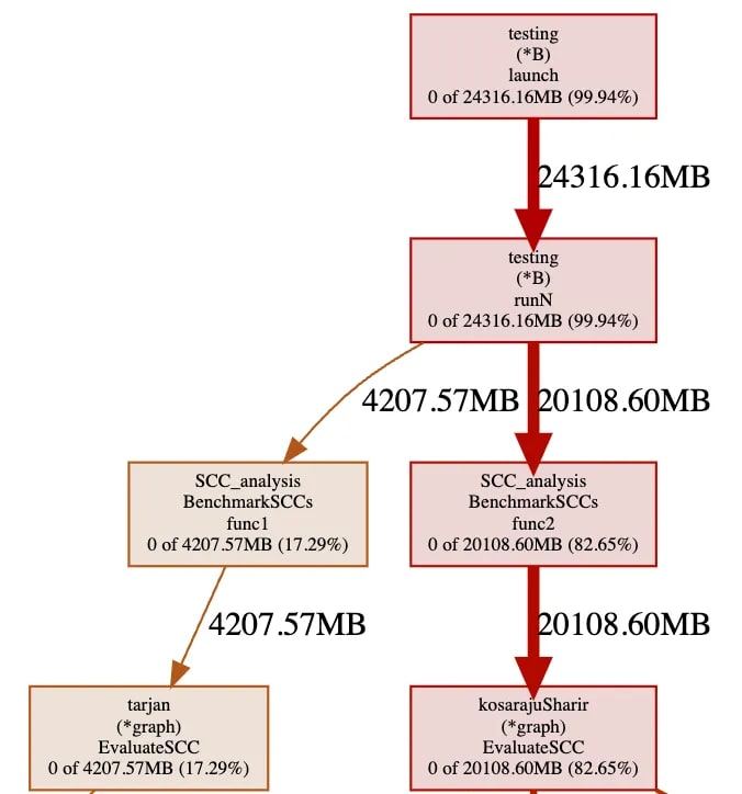
It can be affirmed looking at figure 12 that Kosaraju’s algorithm uses more memory than Tarjan’s algorithm, partly due to a greater number of recursive calls when traversing the base graph (allocating memory on the stack) and also having the pointer in memory of the transposed graph at running time.

To avoid keeping the pointer of the transposed graph in memory, a valid option can be, reversing the original graph at running time, but once the calculations with the transposed graph are finished, the graph must be reversed again in order to achieve the original configuration. With this approach, the graph must be traversed at least twice, doubling the constant execution times.
Conclusions
- Both algorithms perform similarly in general execution time O(V), however Tarjan's approach is more efficient with constant factors of time and memory at execution. In software, everything is a tradeoff, but due to performance challenges, in highly complex distributed systems, any gain in time, even in units of nano seconds, is a significant gain. Under this premise, Tarjan's algorithm is a much more attractive option.
- Tarjan’s algorithm has more development complexity than Kosaraju’s, however both algorithms serve as tools to better understand graph theory and its applicability to the world of technology.
Code implementation
https://github.com/abaron10/Kosaraju_vs_Tarjan
References
- https://blog.revolutionanalytics.com/2010/12/facebooks-social-network-graph.html
- Bang-Jensen & Gutin (2000) p. 19 in the 2007 edition; p. 20 in the 2nd edition (2009). 3.https://mathworld.wolfram.com/WeaklyConnectedDigraph.html#:~:text=A%20weakly%20connected%20digraph%20is,indegree%20of%20at%20least%201.
- https://www.geeksforgeeks.org/topological-sorting/


Latest comments (0)